Feature Engineering 7 - Outliers and Its impact on ML usecases

Outliers and Its impact on Machine Learning!!

What is an outlier?

An outlier is a data point in dataset that is distant from all other observations. A data point that lies outside the overall distribution of the dataset.

What are the reasons for an outlier to exist in a dataset?

1. Variability in data
2. ans experimental error

What are the impacts of having outliers in dataset?

1. It causes various problems during our dtatistical analysis.
2. It may cause a significant impact on the mean and the standard deviation.

What are the criteria to identify an outlier?

1. Data points that falls outside of 1.5 times of IQR above the 3rd quartile or below the 1st quartile. (in case of skewed feature)
2. Data points that falls outside of 3 standard deviations. we can use a z score and if the z score falls outside of 2 standard deviation. (in case of normally distribured feature)

Various ways of finding the outliers.

1. using scatter plots.
2. Using Box plot
3. Using z-score
4. Using the IQR (InterQuantile Range)

Which machine learning models are sensitive to outliers?

1. Naive Bayes Classifier -> No
2. SVM -> No
3. Linear Regression -> Yes
4. Logistic Regression -> Yes
5. Decision Tree regressor or Classifier -> No
6. Ensemble(RF,GBM,XGBoost) -> N0
7. KNN -> No
8. KMeans -> Yes
9. Hierarchical Clustering -> Yes
10. PCA -> Yes
11. LDA -> Yes
12. Neural Network -> Yes

How to treat outliers?

• If outliers are important in our domain, then we should keep it (e.g. Fraud detection) * we should apply those ML algorithm which are not sensitive to outliers in this case
• Else we can remove the same or impute with some other values.

import pandas as pd
import numpy as np
import matplotlib.pyplot as plt
import seaborn as sns
%matplotlib inline

df=pd.read_csv('Datasets/Titanic/train.csv')

df.head()

	PassengerId	Survived	Pclass	Name	Sex	Age	SibSp	Parch	Ticket	Fare	Cabin	Embarked
0	1	0	3	Braund, Mr. Owen Harris	male	22.0	1	0	A/5 21171	7.2500	NaN	S
1	2	1	1	Cumings, Mrs. John Bradley (Florence Briggs Th...	female	38.0	1	0	PC 17599	71.2833	C85	C
2	3	1	3	Heikkinen, Miss. Laina	female	26.0	0	0	STON/O2. 3101282	7.9250	NaN	S
3	4	1	1	Futrelle, Mrs. Jacques Heath (Lily May Peel)	female	35.0	1	0	113803	53.1000	C123	S
4	5	0	3	Allen, Mr. William Henry	male	35.0	0	0	373450	8.0500	NaN	S

df.isna().sum()

PassengerId      0
Survived         0
Pclass           0
Name             0
Sex              0
Age            177
SibSp            0
Parch            0
Ticket           0
Fare             0
Cabin          687
Embarked         2
dtype: int64

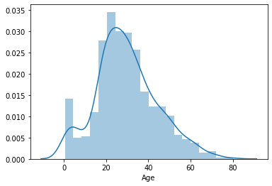
sns.distplot(df.Age.dropna())

<matplotlib.axes._subplots.AxesSubplot at 0x7fd2c6773510>

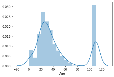
#Just trying to visualise by adding outlier (after replacing NAN values by 110)
sns.distplot(df.Age.fillna(110))

<matplotlib.axes._subplots.AxesSubplot at 0x7fd2c6a3ead0>

• whenever my data follows normal distribution curve, at that time we use technique -> Estimate outliers (or ExtremevalueAnalysis) and we try to find IQR

• when my data is skewed we use different techniques

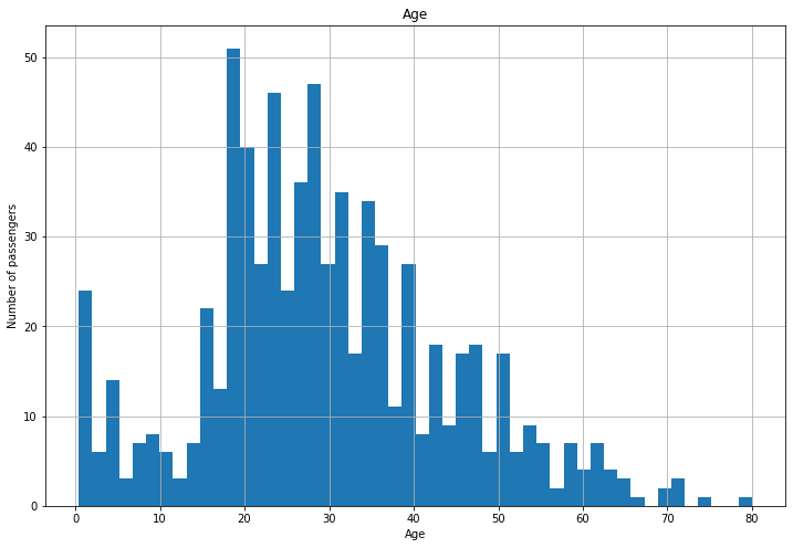
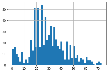
Case 1 :- If features follow Gaussian or normal Distribution

plt.figure(figsize=(12,8))
figure=df.Age.hist(bins=50)
figure.set_title('Age')
figure.set_xlabel('Age')
figure.set_ylabel('Number of passengers')

Text(0, 0.5, 'Number of passengers')

sns.boxplot('Age',data=df)

<matplotlib.axes._subplots.AxesSubplot at 0x7fd2c7a54910>

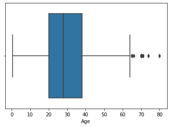
df.Age.describe()

count    714.000000
mean      29.699118
std       14.526497
min        0.420000
25%       20.125000
50%       28.000000
75%       38.000000
max       80.000000
Name: Age, dtype: float64

Assuming “Age” follows Gaussian distribution

# we will calculate boundaries which will differntiate outliers
# Boundary = [mean-3*std_dev,mean+3*std_dev]

age_mean=df.Age.mean()
age_std=df.Age.std()

upper_bound_age=age_mean+3*age_std
lower_bound_age=age_mean-3*age_std

print("upper Boundary:-",upper_bound_age)
print("mean:-",age_mean)
print("lower Boundary:-",lower_bound_age)

upper Boundary:- 73.27860964406095
mean:- 29.69911764705882
lower Boundary:- -13.88037434994331

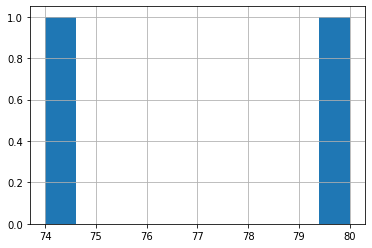
• For Normally distributed dataset we will consider any value which is not between the above mentioned boundary as an outlier.

df.Age[~df.Age.between(lower_bound_age,upper_bound_age)].hist()

<matplotlib.axes._subplots.AxesSubplot at 0x7fd2af73fd10>

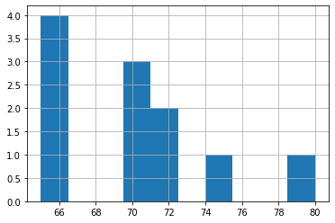
• Below steps we usually follow for Skewed dataset but just how it looks in case of Normally dataset we are trying these

## Lets compute the Inter Quantile Range (IQR) to calculate boundaries
IQR=df.Age.quantile(.75)-df.Age.quantile(.25)
IQR

17.875

lower_bridge=df.Age.quantile(0.25)-(1.5*IQR)
upper_bridge=df.Age.quantile(0.75)+(1.5*IQR)

print("upper Boundary:-",upper_bridge)
print("mean:-",age_mean)
print("lower Boundary:-",lower_bridge)

upper Boundary:- 64.8125
mean:- 29.69911764705882
lower Boundary:- -6.6875

df.Age[~df.Age.between(lower_bridge,upper_bridge)].hist()

<matplotlib.axes._subplots.AxesSubplot at 0x7fd2aff6b910>

# Extreme Outliers
extreme_lower_bridge=df.Age.quantile(0.25)-(3*IQR)
extreme_upper_bridge=df.Age.quantile(0.75)+(3*IQR)

print("upper Boundary:-",extreme_upper_bridge)
print("mean:-",age_mean)
print("lower Boundary:-",extreme_lower_bridge)

upper Boundary:- 91.625
mean:- 29.69911764705882
lower Boundary:- -33.5

• It depends upon domain to decide the boundary for identifying outliers

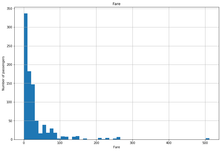
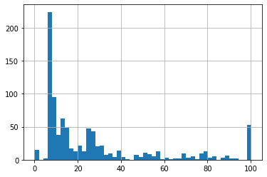
Case 2 :- If features are skewed

plt.figure(figsize=(12,8))
figure=df.Fare.hist(bins=50)
figure.set_title('Fare')
figure.set_xlabel('Fare')
figure.set_ylabel('Number of passengers')

Text(0, 0.5, 'Number of passengers')

sns.boxplot('Fare',data=df)

<matplotlib.axes._subplots.AxesSubplot at 0x7fd2af840d50>

df.Fare.describe()

count    891.000000
mean      32.204208
std       49.693429
min        0.000000
25%        7.910400
50%       14.454200
75%       31.000000
max      512.329200
Name: Fare, dtype: float64

## Lets compute the Inter Quantile Range (IQR) to calculate boundaries
IQR=df.Fare.quantile(.75)-df.Fare.quantile(.25)
IQR

23.0896

fare_mean=df.Fare.mean()

lower_bridge=df.Fare.quantile(0.25)-(1.5*IQR)
upper_bridge=df.Fare.quantile(0.75)+(1.5*IQR)

print("upper Boundary:-",upper_bridge)
print("mean:-",fare_mean)
print("lower Boundary:-",lower_bridge)

upper Boundary:- 65.6344
mean:- 32.2042079685746
lower Boundary:- -26.724

# Extreme Outliers
extreme_lower_bridge=df.Fare.quantile(0.25)-(3*IQR)
extreme_upper_bridge=df.Fare.quantile(0.75)+(3*IQR)
print("upper Boundary:-",extreme_upper_bridge)
print("mean:-",fare_mean)
print("lower Boundary:-",extreme_lower_bridge)

upper Boundary:- 100.2688
mean:- 32.2042079685746
lower Boundary:- -61.358399999999996

• As we can see my data is very much skewed we should take extreme outliers boundary for outliers identification
• It also depends upon domain to decide the boundary for identifying outliers

Aplying Outliers Treatment in Machine Learning models

data=df.copy()

data.loc[data.Age>upper_bound_age,'Age']=int(upper_bound_age)

data.loc[data.Fare>extreme_upper_bridge,'Fare']=extreme_upper_bridge

• We are not replacing outliers below boundaries as we can see are no points below lower boundaries as age and fare can not be negative
• In scenario where there would have been outliers below lower boundary, we would have replaced the same with lower boundary

data.Age.hist(bins=50)

<matplotlib.axes._subplots.AxesSubplot at 0x7fd2b140d650>

data.Fare.hist(bins=50)

<matplotlib.axes._subplots.AxesSubplot at 0x7fd2b16a1390>

from sklearn.model_selection import train_test_split
X_train,X_test,y_train,y_test=train_test_split(data[['Age','Fare']].fillna(0),data.Survived,test_size=0.3,random_state=0)

X_train.shape

(623, 2)

from sklearn.linear_model import LogisticRegression

logit=LogisticRegression()

logit.fit(X_train,y_train)

LogisticRegression()

y_pred=logit.predict(X_test)
y_pred_1=logit.predict_proba(X_test)

from sklearn.metrics import classification_report,confusion_matrix,roc_auc_score,accuracy_score

print("confusion_matrix:-\n",confusion_matrix(y_test,y_pred))
print("\n classification_report:- \n",classification_report(y_test,y_pred))
print("\n accuracy_score:- \n",accuracy_score(y_test,y_pred))
print("\n roc_auc_score:- \n",roc_auc_score(y_test,y_pred_1[:,1]))

confusion_matrix:-
 [[157  11]
 [ 68  32]]

 classification_report:-
               precision    recall  f1-score   support

           0       0.70      0.93      0.80       168
           1       0.74      0.32      0.45       100

    accuracy                           0.71       268
   macro avg       0.72      0.63      0.62       268
weighted avg       0.72      0.71      0.67       268


 accuracy_score:-
 0.7052238805970149

 roc_auc_score:-
 0.7149404761904762

# Random Forest

from sklearn.ensemble import RandomForestClassifier
classifier=RandomForestClassifier()
classifier.fit(X_train,y_train)
y_pred=classifier.predict(X_test)
y_pred_1=classifier.predict_proba(X_test)
print("confusion_matrix:-\n",confusion_matrix(y_test,y_pred))
print("\n classification_report:- \n",classification_report(y_test,y_pred))
print("\n accuracy_score:- \n",accuracy_score(y_test,y_pred))
print("\n roc_auc_score:- \n",roc_auc_score(y_test,y_pred_1[:,1]))

confusion_matrix:-
 [[134  34]
 [ 40  60]]

 classification_report:-
               precision    recall  f1-score   support

           0       0.77      0.80      0.78       168
           1       0.64      0.60      0.62       100

    accuracy                           0.72       268
   macro avg       0.70      0.70      0.70       268
weighted avg       0.72      0.72      0.72       268


 accuracy_score:-
 0.7238805970149254

 roc_auc_score:-
 0.7389880952380952

## Running ML techniques without handling outliers

# Logistic

from sklearn.model_selection import train_test_split
X_train,X_test,y_train,y_test=train_test_split(df[['Age','Fare']].fillna(0),df.Survived,test_size=0.3,random_state=0)
logit=LogisticRegression()
logit.fit(X_train,y_train)
y_pred=logit.predict(X_test)
y_pred_1=logit.predict_proba(X_test)
from sklearn.metrics import classification_report,confusion_matrix,roc_auc_score,accuracy_score
print("confusion_matrix:-\n",confusion_matrix(y_test,y_pred))
print("\n classification_report:- \n",classification_report(y_test,y_pred))
print("\n accuracy_score:- \n",accuracy_score(y_test,y_pred))
print("\n roc_auc_score:- \n",roc_auc_score(y_test,y_pred_1[:,1]))

confusion_matrix:-
 [[161   7]
 [ 75  25]]

 classification_report:-
               precision    recall  f1-score   support

           0       0.68      0.96      0.80       168
           1       0.78      0.25      0.38       100

    accuracy                           0.69       268
   macro avg       0.73      0.60      0.59       268
weighted avg       0.72      0.69      0.64       268


 accuracy_score:-
 0.6940298507462687

 roc_auc_score:-
 0.71375

• As we can see Logistic performs better if we treat outliers

# Random Forest

from sklearn.ensemble import RandomForestClassifier
classifier=RandomForestClassifier()
classifier.fit(X_train,y_train)
y_pred=classifier.predict(X_test)
y_pred_1=classifier.predict_proba(X_test)
print("confusion_matrix:-\n",confusion_matrix(y_test,y_pred))
print("\n classification_report:- \n",classification_report(y_test,y_pred))
print("\n accuracy_score:- \n",accuracy_score(y_test,y_pred))
print("\n roc_auc_score:- \n",roc_auc_score(y_test,y_pred_1[:,1]))

confusion_matrix:-
 [[134  34]
 [ 42  58]]

 classification_report:-
               precision    recall  f1-score   support

           0       0.76      0.80      0.78       168
           1       0.63      0.58      0.60       100

    accuracy                           0.72       268
   macro avg       0.70      0.69      0.69       268
weighted avg       0.71      0.72      0.71       268


 accuracy_score:-
 0.7164179104477612

 roc_auc_score:-
 0.7361011904761905

• As we can see, Random Forest is not much changed even after treating outliers.