

Feature Engineering 5 - Feature Selection Techniques
Feature Selection Techniques
- To reduce the dimensions in models
- Overcoming curse of dimensionality
import pandas as pd
import numpy as np
import matplotlib.pyplot as plt
import seaborn as sns
%matplotlib inline
df=pd.read_csv('Datasets/mobile_dataset.csv')
df.head()
| battery_power | blue | clock_speed | dual_sim | fc | four_g | int_memory | m_dep | mobile_wt | n_cores | ... | px_height | px_width | ram | sc_h | sc_w | talk_time | three_g | touch_screen | wifi | price_range | |
|---|---|---|---|---|---|---|---|---|---|---|---|---|---|---|---|---|---|---|---|---|---|
| 0 | 842 | 0 | 2.2 | 0 | 1 | 0 | 7 | 0.6 | 188 | 2 | ... | 20 | 756 | 2549 | 9 | 7 | 19 | 0 | 0 | 1 | 1 |
| 1 | 1021 | 1 | 0.5 | 1 | 0 | 1 | 53 | 0.7 | 136 | 3 | ... | 905 | 1988 | 2631 | 17 | 3 | 7 | 1 | 1 | 0 | 2 |
| 2 | 563 | 1 | 0.5 | 1 | 2 | 1 | 41 | 0.9 | 145 | 5 | ... | 1263 | 1716 | 2603 | 11 | 2 | 9 | 1 | 1 | 0 | 2 |
| 3 | 615 | 1 | 2.5 | 0 | 0 | 0 | 10 | 0.8 | 131 | 6 | ... | 1216 | 1786 | 2769 | 16 | 8 | 11 | 1 | 0 | 0 | 2 |
| 4 | 1821 | 1 | 1.2 | 0 | 13 | 1 | 44 | 0.6 | 141 | 2 | ... | 1208 | 1212 | 1411 | 8 | 2 | 15 | 1 | 1 | 0 | 1 |
5 rows × 21 columns
df.columns
Index(['battery_power', 'blue', 'clock_speed', 'dual_sim', 'fc', 'four_g',
       'int_memory', 'm_dep', 'mobile_wt', 'n_cores', 'pc', 'px_height',
       'px_width', 'ram', 'sc_h', 'sc_w', 'talk_time', 'three_g',
       'touch_screen', 'wifi', 'price_range'],
      dtype='object')
1. Univariate Selection
- Data should have numerical value (if we have categorial variable in data we can perform feature engineering and convert the same into numerical one).
# Segregating into dependent and independent features
X=df.drop('price_range',axis=1) #Independent Feature
y=df['price_range'] #Dependent Feature
X.head()
| battery_power | blue | clock_speed | dual_sim | fc | four_g | int_memory | m_dep | mobile_wt | n_cores | pc | px_height | px_width | ram | sc_h | sc_w | talk_time | three_g | touch_screen | wifi | |
|---|---|---|---|---|---|---|---|---|---|---|---|---|---|---|---|---|---|---|---|---|
| 0 | 842 | 0 | 2.2 | 0 | 1 | 0 | 7 | 0.6 | 188 | 2 | 2 | 20 | 756 | 2549 | 9 | 7 | 19 | 0 | 0 | 1 |
| 1 | 1021 | 1 | 0.5 | 1 | 0 | 1 | 53 | 0.7 | 136 | 3 | 6 | 905 | 1988 | 2631 | 17 | 3 | 7 | 1 | 1 | 0 |
| 2 | 563 | 1 | 0.5 | 1 | 2 | 1 | 41 | 0.9 | 145 | 5 | 6 | 1263 | 1716 | 2603 | 11 | 2 | 9 | 1 | 1 | 0 |
| 3 | 615 | 1 | 2.5 | 0 | 0 | 0 | 10 | 0.8 | 131 | 6 | 9 | 1216 | 1786 | 2769 | 16 | 8 | 11 | 1 | 0 | 0 |
| 4 | 1821 | 1 | 1.2 | 0 | 13 | 1 | 44 | 0.6 | 141 | 2 | 14 | 1208 | 1212 | 1411 | 8 | 2 | 15 | 1 | 1 | 0 |
y.head()
0    1
1    2
2    2
3    2
4    1
Name: price_range, dtype: int64
from sklearn.feature_selection import SelectKBest # To select top k best features
from sklearn.feature_selection import chi2
X.shape
(2000, 20)
## Apply SelectKBest Algorithm
ordered_rank_features=SelectKBest(score_func=chi2,k=20)
Ordered_feature=ordered_rank_features.fit(X,y)
features_rank=pd.DataFrame(Ordered_feature.scores_,columns=['Score'],index=X.columns).reset_index().rename(columns={'index': 'Feature'})
features_rank.nlargest(10,'Score',keep='all')
| Feature | Score | |
|---|---|---|
| 13 | ram | 931267.519053 |
| 11 | px_height | 17363.569536 |
| 0 | battery_power | 14129.866576 |
| 12 | px_width | 9810.586750 |
| 8 | mobile_wt | 95.972863 |
| 6 | int_memory | 89.839124 |
| 15 | sc_w | 16.480319 |
| 16 | talk_time | 13.236400 |
| 4 | fc | 10.135166 |
| 14 | sc_h | 9.614878 |
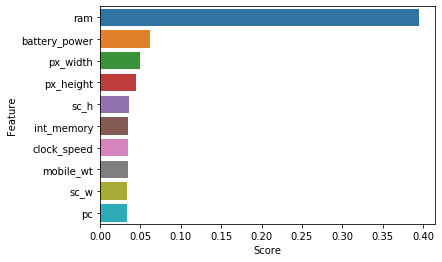
2. Feature Importance
This technique gives us a score for each feature of our data, the higher the score, more relevant it is
from sklearn.ensemble import ExtraTreesClassifier
model=ExtraTreesClassifier()
model.fit(X,y)
/opt/anaconda3/lib/python3.7/site-packages/sklearn/ensemble/forest.py:245: FutureWarning: The default value of n_estimators will change from 10 in version 0.20 to 100 in 0.22.
  "10 in version 0.20 to 100 in 0.22.", FutureWarning)


ExtraTreesClassifier(bootstrap=False, class_weight=None, criterion='gini',
                     max_depth=None, max_features='auto', max_leaf_nodes=None,
                     min_impurity_decrease=0.0, min_impurity_split=None,
                     min_samples_leaf=1, min_samples_split=2,
                     min_weight_fraction_leaf=0.0, n_estimators=10, n_jobs=None,
                     oob_score=False, random_state=None, verbose=0,
                     warm_start=False)
print(model.feature_importances_)
[0.06141965 0.02410379 0.03427029 0.02055451 0.02979936 0.01864498
 0.03502876 0.03265603 0.03416619 0.03286097 0.03296015 0.04391382
 0.05001435 0.39492892 0.03641193 0.03377228 0.03264326 0.01511883
 0.01718066 0.01955127]
ranked_features=pd.DataFrame(model.feature_importances_,columns=['Score'],index=X.columns).reset_index().rename(columns={'index': 'Feature'})
ranked_features
| Feature | Score | |
|---|---|---|
| 0 | battery_power | 0.061420 |
| 1 | blue | 0.024104 |
| 2 | clock_speed | 0.034270 |
| 3 | dual_sim | 0.020555 |
| 4 | fc | 0.029799 |
| 5 | four_g | 0.018645 |
| 6 | int_memory | 0.035029 |
| 7 | m_dep | 0.032656 |
| 8 | mobile_wt | 0.034166 |
| 9 | n_cores | 0.032861 |
| 10 | pc | 0.032960 |
| 11 | px_height | 0.043914 |
| 12 | px_width | 0.050014 |
| 13 | ram | 0.394929 |
| 14 | sc_h | 0.036412 |
| 15 | sc_w | 0.033772 |
| 16 | talk_time | 0.032643 |
| 17 | three_g | 0.015119 |
| 18 | touch_screen | 0.017181 |
| 19 | wifi | 0.019551 |
sns.barplot(x='Score',y='Feature',data=ranked_features.sort_values(['Score'],ascending=False)[:10])
<matplotlib.axes._subplots.AxesSubplot at 0x7fc6380eca50>
3. Correlation
df.corr()
| battery_power | blue | clock_speed | dual_sim | fc | four_g | int_memory | m_dep | mobile_wt | n_cores | ... | px_height | px_width | ram | sc_h | sc_w | talk_time | three_g | touch_screen | wifi | price_range | |
|---|---|---|---|---|---|---|---|---|---|---|---|---|---|---|---|---|---|---|---|---|---|
| battery_power | 1.000000 | 0.011252 | 0.011482 | -0.041847 | 0.033334 | 0.015665 | -0.004004 | 0.034085 | 0.001844 | -0.029727 | ... | 0.014901 | -0.008402 | -0.000653 | -0.029959 | -0.021421 | 0.052510 | 0.011522 | -0.010516 | -0.008343 | 0.200723 |
| blue | 0.011252 | 1.000000 | 0.021419 | 0.035198 | 0.003593 | 0.013443 | 0.041177 | 0.004049 | -0.008605 | 0.036161 | ... | -0.006872 | -0.041533 | 0.026351 | -0.002952 | 0.000613 | 0.013934 | -0.030236 | 0.010061 | -0.021863 | 0.020573 |
| clock_speed | 0.011482 | 0.021419 | 1.000000 | -0.001315 | -0.000434 | -0.043073 | 0.006545 | -0.014364 | 0.012350 | -0.005724 | ... | -0.014523 | -0.009476 | 0.003443 | -0.029078 | -0.007378 | -0.011432 | -0.046433 | 0.019756 | -0.024471 | -0.006606 |
| dual_sim | -0.041847 | 0.035198 | -0.001315 | 1.000000 | -0.029123 | 0.003187 | -0.015679 | -0.022142 | -0.008979 | -0.024658 | ... | -0.020875 | 0.014291 | 0.041072 | -0.011949 | -0.016666 | -0.039404 | -0.014008 | -0.017117 | 0.022740 | 0.017444 |
| fc | 0.033334 | 0.003593 | -0.000434 | -0.029123 | 1.000000 | -0.016560 | -0.029133 | -0.001791 | 0.023618 | -0.013356 | ... | -0.009990 | -0.005176 | 0.015099 | -0.011014 | -0.012373 | -0.006829 | 0.001793 | -0.014828 | 0.020085 | 0.021998 |
| four_g | 0.015665 | 0.013443 | -0.043073 | 0.003187 | -0.016560 | 1.000000 | 0.008690 | -0.001823 | -0.016537 | -0.029706 | ... | -0.019236 | 0.007448 | 0.007313 | 0.027166 | 0.037005 | -0.046628 | 0.584246 | 0.016758 | -0.017620 | 0.014772 |
| int_memory | -0.004004 | 0.041177 | 0.006545 | -0.015679 | -0.029133 | 0.008690 | 1.000000 | 0.006886 | -0.034214 | -0.028310 | ... | 0.010441 | -0.008335 | 0.032813 | 0.037771 | 0.011731 | -0.002790 | -0.009366 | -0.026999 | 0.006993 | 0.044435 |
| m_dep | 0.034085 | 0.004049 | -0.014364 | -0.022142 | -0.001791 | -0.001823 | 0.006886 | 1.000000 | 0.021756 | -0.003504 | ... | 0.025263 | 0.023566 | -0.009434 | -0.025348 | -0.018388 | 0.017003 | -0.012065 | -0.002638 | -0.028353 | 0.000853 |
| mobile_wt | 0.001844 | -0.008605 | 0.012350 | -0.008979 | 0.023618 | -0.016537 | -0.034214 | 0.021756 | 1.000000 | -0.018989 | ... | 0.000939 | 0.000090 | -0.002581 | -0.033855 | -0.020761 | 0.006209 | 0.001551 | -0.014368 | -0.000409 | -0.030302 |
| n_cores | -0.029727 | 0.036161 | -0.005724 | -0.024658 | -0.013356 | -0.029706 | -0.028310 | -0.003504 | -0.018989 | 1.000000 | ... | -0.006872 | 0.024480 | 0.004868 | -0.000315 | 0.025826 | 0.013148 | -0.014733 | 0.023774 | -0.009964 | 0.004399 |
| pc | 0.031441 | -0.009952 | -0.005245 | -0.017143 | 0.644595 | -0.005598 | -0.033273 | 0.026282 | 0.018844 | -0.001193 | ... | -0.018465 | 0.004196 | 0.028984 | 0.004938 | -0.023819 | 0.014657 | -0.001322 | -0.008742 | 0.005389 | 0.033599 |
| px_height | 0.014901 | -0.006872 | -0.014523 | -0.020875 | -0.009990 | -0.019236 | 0.010441 | 0.025263 | 0.000939 | -0.006872 | ... | 1.000000 | 0.510664 | -0.020352 | 0.059615 | 0.043038 | -0.010645 | -0.031174 | 0.021891 | 0.051824 | 0.148858 |
| px_width | -0.008402 | -0.041533 | -0.009476 | 0.014291 | -0.005176 | 0.007448 | -0.008335 | 0.023566 | 0.000090 | 0.024480 | ... | 0.510664 | 1.000000 | 0.004105 | 0.021599 | 0.034699 | 0.006720 | 0.000350 | -0.001628 | 0.030319 | 0.165818 |
| ram | -0.000653 | 0.026351 | 0.003443 | 0.041072 | 0.015099 | 0.007313 | 0.032813 | -0.009434 | -0.002581 | 0.004868 | ... | -0.020352 | 0.004105 | 1.000000 | 0.015996 | 0.035576 | 0.010820 | 0.015795 | -0.030455 | 0.022669 | 0.917046 |
| sc_h | -0.029959 | -0.002952 | -0.029078 | -0.011949 | -0.011014 | 0.027166 | 0.037771 | -0.025348 | -0.033855 | -0.000315 | ... | 0.059615 | 0.021599 | 0.015996 | 1.000000 | 0.506144 | -0.017335 | 0.012033 | -0.020023 | 0.025929 | 0.022986 |
| sc_w | -0.021421 | 0.000613 | -0.007378 | -0.016666 | -0.012373 | 0.037005 | 0.011731 | -0.018388 | -0.020761 | 0.025826 | ... | 0.043038 | 0.034699 | 0.035576 | 0.506144 | 1.000000 | -0.022821 | 0.030941 | 0.012720 | 0.035423 | 0.038711 |
| talk_time | 0.052510 | 0.013934 | -0.011432 | -0.039404 | -0.006829 | -0.046628 | -0.002790 | 0.017003 | 0.006209 | 0.013148 | ... | -0.010645 | 0.006720 | 0.010820 | -0.017335 | -0.022821 | 1.000000 | -0.042688 | 0.017196 | -0.029504 | 0.021859 |
| three_g | 0.011522 | -0.030236 | -0.046433 | -0.014008 | 0.001793 | 0.584246 | -0.009366 | -0.012065 | 0.001551 | -0.014733 | ... | -0.031174 | 0.000350 | 0.015795 | 0.012033 | 0.030941 | -0.042688 | 1.000000 | 0.013917 | 0.004316 | 0.023611 |
| touch_screen | -0.010516 | 0.010061 | 0.019756 | -0.017117 | -0.014828 | 0.016758 | -0.026999 | -0.002638 | -0.014368 | 0.023774 | ... | 0.021891 | -0.001628 | -0.030455 | -0.020023 | 0.012720 | 0.017196 | 0.013917 | 1.000000 | 0.011917 | -0.030411 |
| wifi | -0.008343 | -0.021863 | -0.024471 | 0.022740 | 0.020085 | -0.017620 | 0.006993 | -0.028353 | -0.000409 | -0.009964 | ... | 0.051824 | 0.030319 | 0.022669 | 0.025929 | 0.035423 | -0.029504 | 0.004316 | 0.011917 | 1.000000 | 0.018785 |
| price_range | 0.200723 | 0.020573 | -0.006606 | 0.017444 | 0.021998 | 0.014772 | 0.044435 | 0.000853 | -0.030302 | 0.004399 | ... | 0.148858 | 0.165818 | 0.917046 | 0.022986 | 0.038711 | 0.021859 | 0.023611 | -0.030411 | 0.018785 | 1.000000 |
21 rows × 21 columns
corr=df.corr()
top_features=corr.index
plt.figure(figsize=(20,20))
sns.heatmap(corr,annot=True)
<matplotlib.axes._subplots.AxesSubplot at 0x7fc6385a9f50>
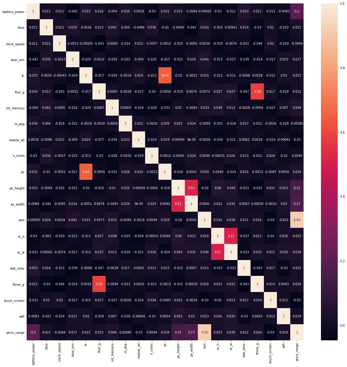
# Removing highly correlated independent features as both will have same kind of impact on dependent variable
threshold=0.5 # This threshold can be decided with domain knowledge
# Find and remove correlated features
def correlation(dataset,threshold):
    col_corr=set() #set of all the names of correlated columns
    corr_matrix=dataset.corr()
    for i in range(len(corr_matrix.columns)):
        for j in range(i):
            if abs(corr_matrix.iloc[i,j])>threshold:
                colname=corr_matrix.columns[i]
                col_corr.add(colname)
    return col_corr
correlation(X,threshold)
{'pc', 'px_width', 'sc_w', 'three_g'}
X.drop(list(correlation(X,threshold)),axis=1).columns
Index(['battery_power', 'blue', 'clock_speed', 'dual_sim', 'fc', 'four_g',
       'int_memory', 'm_dep', 'mobile_wt', 'n_cores', 'px_height', 'ram',
       'sc_h', 'talk_time', 'touch_screen', 'wifi'],
      dtype='object')
- In case of two highly correlated column we usually keep the column which have higher correlated value with dependent variable.
4. Information Gain
Mutual information (MI) between two random variables is a non-negative value, which measures the dependency between the variables. It is equal to zero if and only if two random variables are independent, and higher values mean higher dependency.
from sklearn.feature_selection import mutual_info_classif
mutual_info_classif(X,y)
array([2.76010315e-02, 2.30000049e-03, 1.74688267e-02, 3.30799027e-04,
       0.00000000e+00, 0.00000000e+00, 0.00000000e+00, 1.35307972e-02,
       1.32492474e-02, 0.00000000e+00, 1.31108117e-02, 2.41517674e-02,
       2.75452757e-02, 8.46137627e-01, 9.90067340e-03, 2.28336326e-03,
       0.00000000e+00, 3.42595117e-03, 0.00000000e+00, 0.00000000e+00])
mutual_data=pd.Series(mutual_info_classif(X,y),index=X.columns)
mutual_data.sort_values(ascending=False)
ram              0.849398
battery_power    0.030416
px_width         0.029987
px_height        0.027528
wifi             0.022673
m_dep            0.021102
mobile_wt        0.018650
four_g           0.011000
sc_h             0.010010
pc               0.007630
sc_w             0.006359
touch_screen     0.004327
three_g          0.001078
talk_time        0.000000
int_memory       0.000000
fc               0.000000
dual_sim         0.000000
clock_speed      0.000000
blue             0.000000
n_cores          0.000000
dtype: float64
- we will take only those variable in consideration which have nonzero info gain.
mutual_data[mutual_data.sort_values(ascending=False)>0]
battery_power    0.030416
four_g           0.011000
m_dep            0.021102
mobile_wt        0.018650
pc               0.007630
px_height        0.027528
px_width         0.029987
ram              0.849398
sc_h             0.010010
sc_w             0.006359
three_g          0.001078
touch_screen     0.004327
wifi             0.022673
dtype: float64
5. Dropping Constant Features using VarianceThreshold
- Variance Threshold
-
Feature selector that removes all low-variance features.
-
This feature selection algorithm looks only at the features (X), not the desired outputs (y), and can thus be used for unsupervised learning.
-
data=pd.DataFrame({'A':[1,2,4,1,2,4],
                  'B':[4,5,6,7,8,9],
                  'C':[0,0,0,0,0,0],
                  'D':[1,1,1,1,1,1]})
data
| A | B | C | D | |
|---|---|---|---|---|
| 0 | 1 | 4 | 0 | 1 |
| 1 | 2 | 5 | 0 | 1 |
| 2 | 4 | 6 | 0 | 1 |
| 3 | 1 | 7 | 0 | 1 |
| 4 | 2 | 8 | 0 | 1 |
| 5 | 4 | 9 | 0 | 1 |
from sklearn.feature_selection import VarianceThreshold
var_thres=VarianceThreshold(threshold=0)
var_thres.fit(data)
VarianceThreshold(threshold=0)
var_thres.get_support() #Indicated which of the columns have variance above the threshold value
array([ True, True, False, False])
# Non-Constant Columns
pd.Series(data.columns.tolist())[var_thres.get_support()]
0    A
1    B
dtype: object
# Constant Columns
pd.Series(data.columns.tolist())[~var_thres.get_support()]
2    C
3    D
dtype: object
- Let’s practise on bigger dataset
df5=pd.read_csv('Datasets/Santander_customer_Satisfaction/train.csv',nrows=10000)
df5.shape
(10000, 371)
df5.head()
| ID | var3 | var15 | imp_ent_var16_ult1 | imp_op_var39_comer_ult1 | imp_op_var39_comer_ult3 | imp_op_var40_comer_ult1 | imp_op_var40_comer_ult3 | imp_op_var40_efect_ult1 | imp_op_var40_efect_ult3 | ... | saldo_medio_var33_hace2 | saldo_medio_var33_hace3 | saldo_medio_var33_ult1 | saldo_medio_var33_ult3 | saldo_medio_var44_hace2 | saldo_medio_var44_hace3 | saldo_medio_var44_ult1 | saldo_medio_var44_ult3 | var38 | TARGET | |
|---|---|---|---|---|---|---|---|---|---|---|---|---|---|---|---|---|---|---|---|---|---|
| 0 | 1 | 2 | 23 | 0.0 | 0.0 | 0.0 | 0.0 | 0.0 | 0 | 0 | ... | 0.0 | 0.0 | 0.0 | 0.0 | 0.0 | 0.0 | 0.0 | 0.0 | 39205.170000 | 0 |
| 1 | 3 | 2 | 34 | 0.0 | 0.0 | 0.0 | 0.0 | 0.0 | 0 | 0 | ... | 0.0 | 0.0 | 0.0 | 0.0 | 0.0 | 0.0 | 0.0 | 0.0 | 49278.030000 | 0 |
| 2 | 4 | 2 | 23 | 0.0 | 0.0 | 0.0 | 0.0 | 0.0 | 0 | 0 | ... | 0.0 | 0.0 | 0.0 | 0.0 | 0.0 | 0.0 | 0.0 | 0.0 | 67333.770000 | 0 |
| 3 | 8 | 2 | 37 | 0.0 | 195.0 | 195.0 | 0.0 | 0.0 | 0 | 0 | ... | 0.0 | 0.0 | 0.0 | 0.0 | 0.0 | 0.0 | 0.0 | 0.0 | 64007.970000 | 0 |
| 4 | 10 | 2 | 39 | 0.0 | 0.0 | 0.0 | 0.0 | 0.0 | 0 | 0 | ... | 0.0 | 0.0 | 0.0 | 0.0 | 0.0 | 0.0 | 0.0 | 0.0 | 117310.979016 | 0 |
5 rows × 371 columns
X5=df5.drop('TARGET',axis=1)
y5=df5['TARGET']
from sklearn.model_selection import train_test_split
X_train,X_test,Y_train,y_test=train_test_split(X5,y5,test_size=0.3,random_state=0)
X_train.shape,X_test.shape
((7000, 370), (3000, 370))
# Let's apply variance method
var_thres5=VarianceThreshold(threshold=0)
var_thres5.fit(X_train)
VarianceThreshold(threshold=0)
#Finding number of non constant feature
var_thres5.get_support().sum()
284
# Non-Constant Columns
pd.Series(X_train.columns.tolist())[var_thres5.get_support()].tolist()
['ID',
 'var3',
 'var15',
 'imp_ent_var16_ult1',
 'imp_op_var39_comer_ult1',
 'imp_op_var39_comer_ult3',
 'imp_op_var40_comer_ult1',
 'imp_op_var40_comer_ult3',
 'imp_op_var40_efect_ult1',
 'imp_op_var40_efect_ult3',
 'imp_op_var40_ult1',
 'imp_op_var41_comer_ult1',
 'imp_op_var41_comer_ult3',
 'imp_op_var41_efect_ult1',
 'imp_op_var41_efect_ult3',
 'imp_op_var41_ult1',
 'imp_op_var39_efect_ult1',
 'imp_op_var39_efect_ult3',
 'imp_op_var39_ult1',
 'imp_sal_var16_ult1',
 'ind_var1_0',
 'ind_var1',
 'ind_var5_0',
 'ind_var5',
 'ind_var6_0',
 'ind_var6',
 'ind_var8_0',
 'ind_var8',
 'ind_var12_0',
 'ind_var12',
 'ind_var13_0',
 'ind_var13_corto_0',
 'ind_var13_corto',
 'ind_var13_largo_0',
 'ind_var13_largo',
 'ind_var13',
 'ind_var14_0',
 'ind_var14',
 'ind_var17_0',
 'ind_var17',
 'ind_var19',
 'ind_var20_0',
 'ind_var20',
 'ind_var24_0',
 'ind_var24',
 'ind_var25_cte',
 'ind_var26_0',
 'ind_var26_cte',
 'ind_var26',
 'ind_var25_0',
 'ind_var25',
 'ind_var29_0',
 'ind_var29',
 'ind_var30_0',
 'ind_var30',
 'ind_var31_0',
 'ind_var31',
 'ind_var32_cte',
 'ind_var32_0',
 'ind_var32',
 'ind_var33_0',
 'ind_var33',
 'ind_var37_cte',
 'ind_var37_0',
 'ind_var37',
 'ind_var39_0',
 'ind_var40_0',
 'ind_var40',
 'ind_var41_0',
 'ind_var39',
 'ind_var44_0',
 'ind_var44',
 'num_var1_0',
 'num_var1',
 'num_var4',
 'num_var5_0',
 'num_var5',
 'num_var6_0',
 'num_var6',
 'num_var8_0',
 'num_var8',
 'num_var12_0',
 'num_var12',
 'num_var13_0',
 'num_var13_corto_0',
 'num_var13_corto',
 'num_var13_largo_0',
 'num_var13_largo',
 'num_var13',
 'num_var14_0',
 'num_var14',
 'num_var17_0',
 'num_var17',
 'num_var20_0',
 'num_var20',
 'num_var24_0',
 'num_var24',
 'num_var26_0',
 'num_var26',
 'num_var25_0',
 'num_var25',
 'num_op_var40_hace2',
 'num_op_var40_hace3',
 'num_op_var40_ult1',
 'num_op_var40_ult3',
 'num_op_var41_hace2',
 'num_op_var41_hace3',
 'num_op_var41_ult1',
 'num_op_var41_ult3',
 'num_op_var39_hace2',
 'num_op_var39_hace3',
 'num_op_var39_ult1',
 'num_op_var39_ult3',
 'num_var29_0',
 'num_var29',
 'num_var30_0',
 'num_var30',
 'num_var31_0',
 'num_var31',
 'num_var32_0',
 'num_var32',
 'num_var33_0',
 'num_var33',
 'num_var35',
 'num_var37_med_ult2',
 'num_var37_0',
 'num_var37',
 'num_var39_0',
 'num_var40_0',
 'num_var40',
 'num_var41_0',
 'num_var39',
 'num_var42_0',
 'num_var42',
 'num_var44_0',
 'num_var44',
 'saldo_var1',
 'saldo_var5',
 'saldo_var6',
 'saldo_var8',
 'saldo_var12',
 'saldo_var13_corto',
 'saldo_var13_largo',
 'saldo_var13',
 'saldo_var14',
 'saldo_var17',
 'saldo_var20',
 'saldo_var24',
 'saldo_var26',
 'saldo_var25',
 'saldo_var29',
 'saldo_var30',
 'saldo_var31',
 'saldo_var32',
 'saldo_var33',
 'saldo_var37',
 'saldo_var40',
 'saldo_var42',
 'saldo_var44',
 'var36',
 'delta_imp_aport_var13_1y3',
 'delta_imp_aport_var17_1y3',
 'delta_imp_aport_var33_1y3',
 'delta_imp_compra_var44_1y3',
 'delta_imp_reemb_var13_1y3',
 'delta_imp_trasp_var17_in_1y3',
 'delta_imp_trasp_var33_in_1y3',
 'delta_imp_venta_var44_1y3',
 'delta_num_aport_var13_1y3',
 'delta_num_aport_var17_1y3',
 'delta_num_aport_var33_1y3',
 'delta_num_compra_var44_1y3',
 'delta_num_reemb_var13_1y3',
 'delta_num_trasp_var17_in_1y3',
 'delta_num_trasp_var33_in_1y3',
 'delta_num_venta_var44_1y3',
 'imp_aport_var13_hace3',
 'imp_aport_var13_ult1',
 'imp_aport_var17_hace3',
 'imp_aport_var17_ult1',
 'imp_aport_var33_hace3',
 'imp_aport_var33_ult1',
 'imp_var7_recib_ult1',
 'imp_compra_var44_hace3',
 'imp_compra_var44_ult1',
 'imp_reemb_var13_ult1',
 'imp_var43_emit_ult1',
 'imp_trans_var37_ult1',
 'imp_trasp_var17_in_ult1',
 'imp_trasp_var33_in_ult1',
 'imp_venta_var44_ult1',
 'ind_var7_recib_ult1',
 'ind_var10_ult1',
 'ind_var10cte_ult1',
 'ind_var9_cte_ult1',
 'ind_var9_ult1',
 'ind_var43_emit_ult1',
 'ind_var43_recib_ult1',
 'var21',
 'num_aport_var13_hace3',
 'num_aport_var13_ult1',
 'num_aport_var17_hace3',
 'num_aport_var17_ult1',
 'num_aport_var33_hace3',
 'num_aport_var33_ult1',
 'num_var7_recib_ult1',
 'num_compra_var44_hace3',
 'num_compra_var44_ult1',
 'num_ent_var16_ult1',
 'num_var22_hace2',
 'num_var22_hace3',
 'num_var22_ult1',
 'num_var22_ult3',
 'num_med_var22_ult3',
 'num_med_var45_ult3',
 'num_meses_var5_ult3',
 'num_meses_var8_ult3',
 'num_meses_var12_ult3',
 'num_meses_var13_corto_ult3',
 'num_meses_var13_largo_ult3',
 'num_meses_var17_ult3',
 'num_meses_var29_ult3',
 'num_meses_var33_ult3',
 'num_meses_var39_vig_ult3',
 'num_meses_var44_ult3',
 'num_op_var39_comer_ult1',
 'num_op_var39_comer_ult3',
 'num_op_var40_comer_ult1',
 'num_op_var40_comer_ult3',
 'num_op_var40_efect_ult1',
 'num_op_var40_efect_ult3',
 'num_op_var41_comer_ult1',
 'num_op_var41_comer_ult3',
 'num_op_var41_efect_ult1',
 'num_op_var41_efect_ult3',
 'num_op_var39_efect_ult1',
 'num_op_var39_efect_ult3',
 'num_reemb_var13_ult1',
 'num_sal_var16_ult1',
 'num_var43_emit_ult1',
 'num_var43_recib_ult1',
 'num_trasp_var11_ult1',
 'num_trasp_var17_in_ult1',
 'num_trasp_var33_in_ult1',
 'num_venta_var44_ult1',
 'num_var45_hace2',
 'num_var45_hace3',
 'num_var45_ult1',
 'num_var45_ult3',
 'saldo_medio_var5_hace2',
 'saldo_medio_var5_hace3',
 'saldo_medio_var5_ult1',
 'saldo_medio_var5_ult3',
 'saldo_medio_var8_hace2',
 'saldo_medio_var8_hace3',
 'saldo_medio_var8_ult1',
 'saldo_medio_var8_ult3',
 'saldo_medio_var12_hace2',
 'saldo_medio_var12_hace3',
 'saldo_medio_var12_ult1',
 'saldo_medio_var12_ult3',
 'saldo_medio_var13_corto_hace2',
 'saldo_medio_var13_corto_hace3',
 'saldo_medio_var13_corto_ult1',
 'saldo_medio_var13_corto_ult3',
 'saldo_medio_var13_largo_hace2',
 'saldo_medio_var13_largo_hace3',
 'saldo_medio_var13_largo_ult1',
 'saldo_medio_var13_largo_ult3',
 'saldo_medio_var17_hace2',
 'saldo_medio_var17_hace3',
 'saldo_medio_var17_ult1',
 'saldo_medio_var17_ult3',
 'saldo_medio_var29_ult1',
 'saldo_medio_var29_ult3',
 'saldo_medio_var33_hace2',
 'saldo_medio_var33_hace3',
 'saldo_medio_var33_ult1',
 'saldo_medio_var33_ult3',
 'saldo_medio_var44_hace2',
 'saldo_medio_var44_hace3',
 'saldo_medio_var44_ult1',
 'saldo_medio_var44_ult3',
 'var38']
# Constant Columns
const_col=pd.Series(X_train.columns.tolist())[~var_thres5.get_support()].tolist()
X_train.drop(const_col,axis=1)
| ID | var3 | var15 | imp_ent_var16_ult1 | imp_op_var39_comer_ult1 | imp_op_var39_comer_ult3 | imp_op_var40_comer_ult1 | imp_op_var40_comer_ult3 | imp_op_var40_efect_ult1 | imp_op_var40_efect_ult3 | ... | saldo_medio_var29_ult3 | saldo_medio_var33_hace2 | saldo_medio_var33_hace3 | saldo_medio_var33_ult1 | saldo_medio_var33_ult3 | saldo_medio_var44_hace2 | saldo_medio_var44_hace3 | saldo_medio_var44_ult1 | saldo_medio_var44_ult3 | var38 | |
|---|---|---|---|---|---|---|---|---|---|---|---|---|---|---|---|---|---|---|---|---|---|
| 7681 | 15431 | 2 | 42 | 840.0 | 4477.02 | 4989.54 | 0.0 | 0.0 | 0 | 0 | ... | 0.0 | 0.0 | 0.0 | 0.0 | 0.0 | 0.0 | 0.0 | 0.0 | 0.0 | 37491.21 |
| 9031 | 18181 | 2 | 31 | 0.0 | 52.32 | 52.32 | 0.0 | 0.0 | 0 | 0 | ... | 0.0 | 0.0 | 0.0 | 0.0 | 0.0 | 0.0 | 0.0 | 0.0 | 0.0 | 106685.94 |
| 3691 | 7411 | 2 | 51 | 0.0 | 0.00 | 0.00 | 0.0 | 0.0 | 0 | 0 | ... | 0.0 | 0.0 | 0.0 | 0.0 | 0.0 | 0.0 | 0.0 | 0.0 | 0.0 | 66144.66 |
| 202 | 407 | 2 | 36 | 0.0 | 0.00 | 0.00 | 0.0 | 0.0 | 0 | 0 | ... | 0.0 | 0.0 | 0.0 | 0.0 | 0.0 | 0.0 | 0.0 | 0.0 | 0.0 | 92121.36 |
| 5625 | 11280 | 2 | 23 | 0.0 | 0.00 | 0.00 | 0.0 | 0.0 | 0 | 0 | ... | 0.0 | 0.0 | 0.0 | 0.0 | 0.0 | 0.0 | 0.0 | 0.0 | 0.0 | 74650.83 |
| ... | ... | ... | ... | ... | ... | ... | ... | ... | ... | ... | ... | ... | ... | ... | ... | ... | ... | ... | ... | ... | ... |
| 9225 | 18564 | 2 | 33 | 0.0 | 0.00 | 0.00 | 0.0 | 0.0 | 0 | 0 | ... | 0.0 | 0.0 | 0.0 | 0.0 | 0.0 | 0.0 | 0.0 | 0.0 | 0.0 | 117547.89 |
| 4859 | 9723 | 2 | 24 | 0.0 | 0.00 | 0.00 | 0.0 | 0.0 | 0 | 0 | ... | 0.0 | 0.0 | 0.0 | 0.0 | 0.0 | 0.0 | 0.0 | 0.0 | 0.0 | 71050.83 |
| 3264 | 6557 | 2 | 24 | 0.0 | 0.00 | 0.00 | 0.0 | 0.0 | 0 | 0 | ... | 0.0 | 0.0 | 0.0 | 0.0 | 0.0 | 0.0 | 0.0 | 0.0 | 0.0 | 141069.33 |
| 9845 | 19796 | 2 | 38 | 0.0 | 0.00 | 0.00 | 0.0 | 0.0 | 0 | 0 | ... | 0.0 | 0.0 | 0.0 | 0.0 | 0.0 | 0.0 | 0.0 | 0.0 | 0.0 | 86412.15 |
| 2732 | 5441 | 2 | 23 | 0.0 | 0.00 | 0.00 | 0.0 | 0.0 | 0 | 0 | ... | 0.0 | 0.0 | 0.0 | 0.0 | 0.0 | 0.0 | 0.0 | 0.0 | 0.0 | 45985.68 |
7000 rows × 284 columns