Feature Engineering 4 - Standardisation and Transformation

Transformation of Variable

• Why transformation of features are required?
  1. Linear Regression - Gradient Descent – Global Minima
     • To acheieve global minima easily we need to transform our data
  2. Algorithm like KNN, K means, hierarchical Clustering. – Euclidian distance involved in these algorithm
     • if differnece in values between variable is large then calculating distance between them will take time
     • Before tranfromation (Time taking)
       • P1= (X1,Y1)=(3,70) P2= (X2,Y2)=(2,50)
     • After transformation or scaling (Less time consuming)
       • P1 = (.03,0.7) P2 = (.02,0.5)
     • It enchances the performance of model
  3. Deep Learning
  • ANN –> Global Minima,Gradient Descent, Back propogation
  • CNN
  • RNN

Types of Transformations :-

1. Normalization and Standardisation (StandardScaler)
2. Scaling to Minimum and Maximum values (MinMaxScaler)
3. Sacaling to Median and Quantiles (RobustScaler)
4. Gaussian Transformation
    a. Logarithmic Transformation
    b. Reciprocal Transformation
    c. Square Root Transformation
    d. Exponential Transformation
    e. Box-Cox Transformation

import pandas as pd
import numpy as np
import matplotlib.pyplot as plt
import seaborn as sns
%matplotlib inline

1. Standardisation

We try to bring all the variables or features to similar scale.

• Standardization means centering the variable at zero. (Mean=0 , std_dev=1)
• Z=(X-X_mean)/X_stdDev
• If there is an outlier there will be impact in standardization

df1=pd.read_csv('Datasets/Titanic/train.csv',usecols=['Pclass','Age','Fare','Survived'])
df1.head()

	Survived	Pclass	Age	Fare
0	0	3	22.0	7.2500
1	1	1	38.0	71.2833
2	1	3	26.0	7.9250
3	1	1	35.0	53.1000
4	0	3	35.0	8.0500

df1.isna().sum()

Survived      0
Pclass        0
Age         177
Fare          0
dtype: int64

df1.Age.fillna(df1.Age.median(),inplace=True)

Standardization : We use StandardScaler from slearn library

from sklearn.preprocessing import StandardScaler

scaler=StandardScaler()
df1_scaled=scaler.fit_transform(df1)

pd.DataFrame(df1_scaled)

	0	1	2	3
0	-0.789272	0.827377	-0.565736	-0.502445
1	1.266990	-1.566107	0.663861	0.786845
2	1.266990	0.827377	-0.258337	-0.488854
3	1.266990	-1.566107	0.433312	0.420730
4	-0.789272	0.827377	0.433312	-0.486337
...	...	...	...	...
886	-0.789272	-0.369365	-0.181487	-0.386671
887	1.266990	-1.566107	-0.796286	-0.044381
888	-0.789272	0.827377	-0.104637	-0.176263
889	1.266990	-1.566107	-0.258337	-0.044381
890	-0.789272	0.827377	0.202762	-0.492378

891 rows × 4 columns

plt.hist(df1_scaled[:,2],bins=20)

(array([ 40.,  14.,  15.,  31.,  79.,  98., 262.,  84.,  73.,  45.,  35.,
         35.,  29.,  16.,  13.,  11.,   4.,   5.,   1.,   1.]),
 array([-2.22415608, -1.91837055, -1.61258503, -1.3067995 , -1.00101397,
        -0.69522845, -0.38944292, -0.08365739,  0.22212813,  0.52791366,
         0.83369919,  1.13948471,  1.44527024,  1.75105577,  2.05684129,
         2.36262682,  2.66841235,  2.97419787,  3.2799834 ,  3.58576892,
         3.89155445]),
 <a list of 20 Patch objects>)

plt.hist(df1_scaled[:,3],bins=20)

(array([562., 170.,  67.,  39.,  15.,  16.,   2.,   0.,   9.,   2.,   6.,
          0.,   0.,   0.,   0.,   0.,   0.,   0.,   0.,   3.]),
 array([-0.64842165, -0.13264224,  0.38313716,  0.89891657,  1.41469598,
         1.93047539,  2.4462548 ,  2.96203421,  3.47781362,  3.99359303,
         4.50937244,  5.02515184,  5.54093125,  6.05671066,  6.57249007,
         7.08826948,  7.60404889,  8.1198283 ,  8.63560771,  9.15138712,
         9.66716653]),
 <a list of 20 Patch objects>)

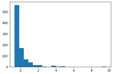
• the above graph is right skewed

2. Min-Max Scaling

• Min Max Scaling scales the values between 0 to 1.
• X_scaled = (X-X_min)/(X_max-X_min)

from sklearn.preprocessing import MinMaxScaler

min_max=MinMaxScaler()

df2=df1.copy()

df2.head()

	Survived	Pclass	Age	Fare
0	0	3	22.0	7.2500
1	1	1	38.0	71.2833
2	1	3	26.0	7.9250
3	1	1	35.0	53.1000
4	0	3	35.0	8.0500

df_minmax=pd.DataFrame(min_max.fit_transform(df2),columns=df2.columns)

df_minmax

	Survived	Pclass	Age	Fare
0	0.0	1.0	0.271174	0.014151
1	1.0	0.0	0.472229	0.139136
2	1.0	1.0	0.321438	0.015469
3	1.0	0.0	0.434531	0.103644
4	0.0	1.0	0.434531	0.015713
...	...	...	...	...
886	0.0	0.5	0.334004	0.025374
887	1.0	0.0	0.233476	0.058556
888	0.0	1.0	0.346569	0.045771
889	1.0	0.0	0.321438	0.058556
890	0.0	1.0	0.396833	0.015127

891 rows × 4 columns

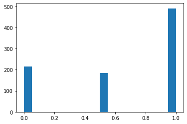
plt.hist(df_minmax['Pclass'],bins=20)

(array([216.,   0.,   0.,   0.,   0.,   0.,   0.,   0.,   0.,   0., 184.,
          0.,   0.,   0.,   0.,   0.,   0.,   0.,   0., 491.]),
 array([0.  , 0.05, 0.1 , 0.15, 0.2 , 0.25, 0.3 , 0.35, 0.4 , 0.45, 0.5 ,
        0.55, 0.6 , 0.65, 0.7 , 0.75, 0.8 , 0.85, 0.9 , 0.95, 1.  ]),
 <a list of 20 Patch objects>)

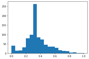
plt.hist(df_minmax['Age'],bins=20)

(array([ 40.,  14.,  15.,  31.,  79.,  98., 262.,  84.,  73.,  45.,  35.,
         35.,  29.,  16.,  13.,  11.,   4.,   5.,   1.,   1.]),
 array([0.  , 0.05, 0.1 , 0.15, 0.2 , 0.25, 0.3 , 0.35, 0.4 , 0.45, 0.5 ,
        0.55, 0.6 , 0.65, 0.7 , 0.75, 0.8 , 0.85, 0.9 , 0.95, 1.  ]),
 <a list of 20 Patch objects>)

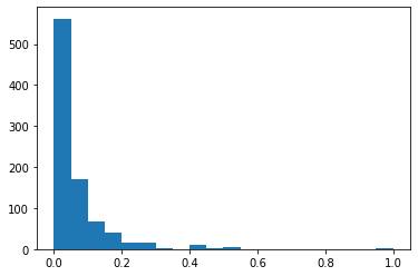
plt.hist(df_minmax['Fare'],bins=20)

(array([562., 170.,  67.,  39.,  15.,  16.,   2.,   0.,   9.,   2.,   6.,
          0.,   0.,   0.,   0.,   0.,   0.,   0.,   0.,   3.]),
 array([0.  , 0.05, 0.1 , 0.15, 0.2 , 0.25, 0.3 , 0.35, 0.4 , 0.45, 0.5 ,
        0.55, 0.6 , 0.65, 0.7 , 0.75, 0.8 , 0.85, 0.9 , 0.95, 1.  ]),
 <a list of 20 Patch objects>)

3. Robust Scaler

• it is used to scale the featured to median and quantiles

• Scaling using median and quantiles consists of subtracting the median to all the observations, and then dividing by the interquantile difference(IQR). The interquantile difference is the difference between 75th and 25th quantile.

• IQR = 75th Quantile - 25th Quantile

• X_scaled= (X-X.median)/IQR

• If the distribution of the variable is skewed, perhaps it better to scale using median and quantiles method which is more robust to presence of outliers

from sklearn.preprocessing import RobustScaler

rob_scl=RobustScaler()

df3=df1.copy()

df3.quantile([.25,.5,.75])

	Survived	Pclass	Age	Fare
0.25	0.0	2.0	22.0	7.9104
0.50	0.0	3.0	28.0	14.4542
0.75	1.0	3.0	35.0	31.0000

df3_robust_scaled=pd.DataFrame(rob_scl.fit_transform(df3),columns=df3.columns)

df3_robust_scaled

	Survived	Pclass	Age	Fare
0	0.0	0.0	-0.461538	-0.312011
1	1.0	-2.0	0.769231	2.461242
2	1.0	0.0	-0.153846	-0.282777
3	1.0	-2.0	0.538462	1.673732
4	0.0	0.0	0.538462	-0.277363
...	...	...	...	...
886	0.0	-1.0	-0.076923	-0.062981
887	1.0	-2.0	-0.692308	0.673281
888	0.0	0.0	0.000000	0.389604
889	1.0	-2.0	-0.153846	0.673281
890	0.0	0.0	0.307692	-0.290356

891 rows × 4 columns

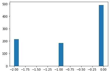
plt.hist(df3_robust_scaled['Pclass'],bins=20)

(array([216.,   0.,   0.,   0.,   0.,   0.,   0.,   0.,   0.,   0., 184.,
          0.,   0.,   0.,   0.,   0.,   0.,   0.,   0., 491.]),
 array([-2. , -1.9, -1.8, -1.7, -1.6, -1.5, -1.4, -1.3, -1.2, -1.1, -1. ,
        -0.9, -0.8, -0.7, -0.6, -0.5, -0.4, -0.3, -0.2, -0.1,  0. ]),
 <a list of 20 Patch objects>)

plt.hist(df3_robust_scaled['Age'],bins=20)

(array([ 40.,  14.,  15.,  31.,  79.,  98., 262.,  84.,  73.,  45.,  35.,
         35.,  29.,  16.,  13.,  11.,   4.,   5.,   1.,   1.]),
 array([-2.12153846, -1.81546154, -1.50938462, -1.20330769, -0.89723077,
        -0.59115385, -0.28507692,  0.021     ,  0.32707692,  0.63315385,
         0.93923077,  1.24530769,  1.55138462,  1.85746154,  2.16353846,
         2.46961538,  2.77569231,  3.08176923,  3.38784615,  3.69392308,
         4.        ]),
 <a list of 20 Patch objects>)

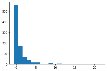
plt.hist(df3_robust_scaled['Fare'],bins=20)

(array([562., 170.,  67.,  39.,  15.,  16.,   2.,   0.,   9.,   2.,   6.,
          0.,   0.,   0.,   0.,   0.,   0.,   0.,   0.,   3.]),
 array([-0.62600478,  0.48343237,  1.59286952,  2.70230667,  3.81174382,
         4.92118096,  6.03061811,  7.14005526,  8.24949241,  9.35892956,
        10.46836671, 11.57780386, 12.68724101, 13.79667816, 14.90611531,
        16.01555246, 17.12498961, 18.23442675, 19.3438639 , 20.45330105,
        21.5627382 ]),
 <a list of 20 Patch objects>)

4. Gaussian Transformation

• Why is Gaussian Distribution Important?
  • Gaussian distribution is ubiquitous because a dataset with finite variance turns into Gaussian as long as dataset with independent feature-probabilities is allowed to grow in size. Gaussian distribution is the most important probability distribution in statistics because it fits many natural phenomena like age, height, test-scores, IQ scores, sum of the rolls of two dices and so on.
  • Datasets with Gaussian distributions makes applicable to a variety of methods that fall under parametric statistics. The methods such as propagation of uncertainty and least squares parameter fitting that make a data-scientist life easy are applicable only to datasets with normal or normal-like distributions.
  • Conclusions and summaries derived from such analysis are intuitive and easy to explain to audiences with basic knowledge of statistics.

Note :- Standardization is not a type of Gaussian tranformation

• If my features are not normally distributed, we apply some mathematical calculation to convert the same into Gaussian distribution or normal distribution.
• Why Normal distribution is required?
  • Some of the ML algorithm (Like Linear and logistic regression ) performs well if my data is normally distributed as the assume that data is normally distributed.

df4=pd.read_csv('Datasets/Titanic/train.csv',usecols=['Age','Fare','Survived'])
df4.head()

	Survived	Age	Fare
0	0	22.0	7.2500
1	1	38.0	71.2833
2	1	26.0	7.9250
3	1	35.0	53.1000
4	0	35.0	8.0500

df4.Age.fillna(df4.Age.median(),inplace=True)

df4.isna().sum()

Survived    0
Age         0
Fare        0
dtype: int64

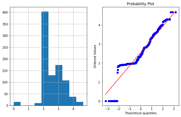
If we want to check whether feature is gaussian or normal distributed , we can use *QQ plot

import scipy.stats as stat
import pylab

def plot_data(df,feature):
    plt.figure(figsize=(10,6))
    plt.subplot(1,2,1)
    df[feature].hist()
    plt.subplot(1,2,2)
    stat.probplot(df[feature],dist='norm',plot=pylab)
    plt.show()

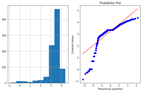
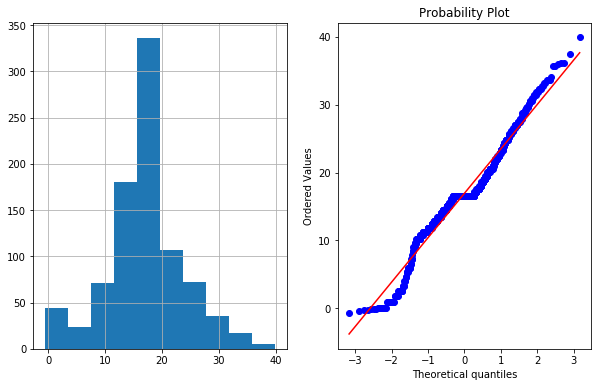
plot_data(df4,'Age')

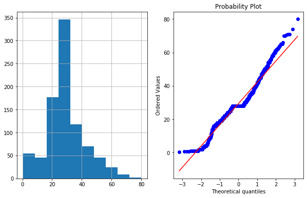
• In right figurte (QQ Plot) The data (on Y-axis) should fall on straight line if it is normally distributed or follow Gaussian distribution.

4a. Logarithmic Transformation

df4['Age_log']=np.log(df4['Age'])
plot_data(df4,'Age_log')

• As we can see log transformation didn’t worked well in this case

4b. Reciprocal Transformation

df4['Age_reciprocal']=1/df4.Age
plot_data(df4,'Age_reciprocal')

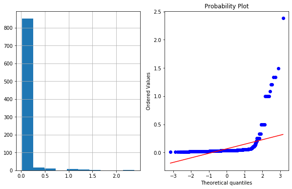
4c. Square Root Transformation

df4['Age_sq_root']=df4.Age**(1/2)

plot_data(df4,'Age_sq_root')

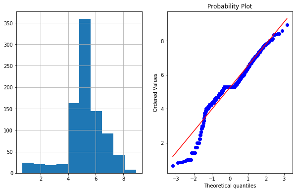
4d. Exponential Transformation

exp(df4.Age)

---------------------------------------------------------------------------

NameError                                 Traceback (most recent call last)

<ipython-input-86-195cdc59ab32> in <module>
----> 1 exp(df4.Age)


NameError: name 'exp' is not defined

df4['Age_exponential']=df4.Age**(1/1.2)  # e**x=x**(1/1/2)

plot_data(df4,'Age_exponential')

4e. Box-Cox Transformation

• The Box-Cox transformation is defined as:

  • T(Y) = (Y exp(Lambda)-1)/Lambda
  • where Y is the response Variable (Feature value) and “Lambda” is the transformation parameter. “Lambda” varies from -5 to 5. In the transformation, all the values of “Lambda” are considered and the optimal value for a given variable is selected.
  • “https://www.spcforexcel.com/knowledge/basic-statistics/box-cox-transformation” refer this for more details.

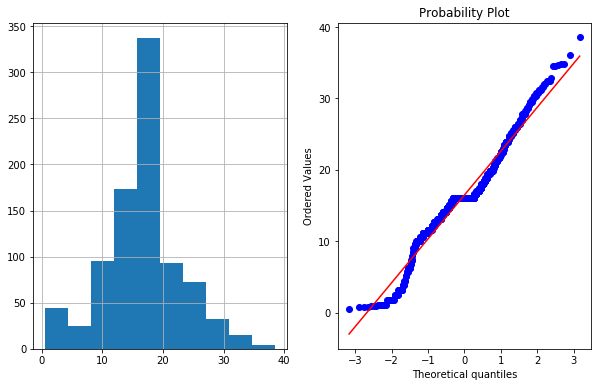
df4['Age_boxcox'],parameters=stat.boxcox(df4['Age'])

parameters

0.7964531473656952

plot_data(df4,'Age_boxcox')

• Notes :-
  • We can apply all the Gaussian distribution using for loop and then pick the best one.
  • We can apply standardization and normalization transformation after Gaussian transformation or vice versa.

## Fare
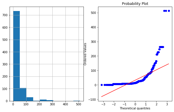
plot_data(df4,'Fare')

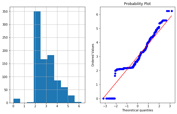
df4['Fare_log']=np.log1p(df4['Fare']) # As fare had 0 values we used log1p insted of log --> log1p(x) =log(1+x)
plot_data(df4,'Fare_log')

df4['Fare_boxcox'],parameters=stat.boxcox(df4['Fare']+1)
plot_data(df4,'Fare_boxcox')