Feature Engineering 2 - Missing values - Categorial

Missing Values - Feature Engineering - Categorial Variable

import pandas as pd
import numpy as np
import matplotlib.pyplot as plt
import seaborn as sns
%matplotlib inline

How to handle categorial missing values

df=pd.read_csv('Datasets/House_prices/train.csv')
df.head()

	Id	MSSubClass	MSZoning	LotFrontage	LotArea	Street	Alley	LotShape	LandContour	Utilities	...	PoolArea	PoolQC	Fence	MiscFeature	MiscVal	MoSold	YrSold	SaleType	SaleCondition	SalePrice
0	1	60	RL	65.0	8450	Pave	NaN	Reg	Lvl	AllPub	...	0	NaN	NaN	NaN	0	2	2008	WD	Normal	208500
1	2	20	RL	80.0	9600	Pave	NaN	Reg	Lvl	AllPub	...	0	NaN	NaN	NaN	0	5	2007	WD	Normal	181500
2	3	60	RL	68.0	11250	Pave	NaN	IR1	Lvl	AllPub	...	0	NaN	NaN	NaN	0	9	2008	WD	Normal	223500
3	4	70	RL	60.0	9550	Pave	NaN	IR1	Lvl	AllPub	...	0	NaN	NaN	NaN	0	2	2006	WD	Abnorml	140000
4	5	60	RL	84.0	14260	Pave	NaN	IR1	Lvl	AllPub	...	0	NaN	NaN	NaN	0	12	2008	WD	Normal	250000

5 rows × 81 columns

df.columns

Index(['Id', 'MSSubClass', 'MSZoning', 'LotFrontage', 'LotArea', 'Street',
       'Alley', 'LotShape', 'LandContour', 'Utilities', 'LotConfig',
       'LandSlope', 'Neighborhood', 'Condition1', 'Condition2', 'BldgType',
       'HouseStyle', 'OverallQual', 'OverallCond', 'YearBuilt', 'YearRemodAdd',
       'RoofStyle', 'RoofMatl', 'Exterior1st', 'Exterior2nd', 'MasVnrType',
       'MasVnrArea', 'ExterQual', 'ExterCond', 'Foundation', 'BsmtQual',
       'BsmtCond', 'BsmtExposure', 'BsmtFinType1', 'BsmtFinSF1',
       'BsmtFinType2', 'BsmtFinSF2', 'BsmtUnfSF', 'TotalBsmtSF', 'Heating',
       'HeatingQC', 'CentralAir', 'Electrical', '1stFlrSF', '2ndFlrSF',
       'LowQualFinSF', 'GrLivArea', 'BsmtFullBath', 'BsmtHalfBath', 'FullBath',
       'HalfBath', 'BedroomAbvGr', 'KitchenAbvGr', 'KitchenQual',
       'TotRmsAbvGrd', 'Functional', 'Fireplaces', 'FireplaceQu', 'GarageType',
       'GarageYrBlt', 'GarageFinish', 'GarageCars', 'GarageArea', 'GarageQual',
       'GarageCond', 'PavedDrive', 'WoodDeckSF', 'OpenPorchSF',
       'EnclosedPorch', '3SsnPorch', 'ScreenPorch', 'PoolArea', 'PoolQC',
       'Fence', 'MiscFeature', 'MiscVal', 'MoSold', 'YrSold', 'SaleType',
       'SaleCondition', 'SalePrice'],
      dtype='object')

df[df.columns[df.isna().sum()>0]].isna().mean().sort_values()

Electrical      0.000685
MasVnrType      0.005479
MasVnrArea      0.005479
BsmtQual        0.025342
BsmtCond        0.025342
BsmtFinType1    0.025342
BsmtExposure    0.026027
BsmtFinType2    0.026027
GarageCond      0.055479
GarageQual      0.055479
GarageFinish    0.055479
GarageType      0.055479
GarageYrBlt     0.055479
LotFrontage     0.177397
FireplaceQu     0.472603
Fence           0.807534
Alley           0.937671
MiscFeature     0.963014
PoolQC          0.995205
dtype: float64

1. Frequent categories imputation

df1=pd.read_csv('Datasets/House_prices/train.csv',usecols=['BsmtQual','FireplaceQu','GarageType','SalePrice'])

df1.head()

	BsmtQual	FireplaceQu	GarageType	SalePrice
0	Gd	NaN	Attchd	208500
1	Gd	TA	Attchd	181500
2	Gd	TA	Attchd	223500
3	TA	Gd	Detchd	140000
4	Gd	TA	Attchd	250000

df1.isna().sum()

BsmtQual        37
FireplaceQu    690
GarageType      81
SalePrice        0
dtype: int64

df1.isna().mean().sort_values(ascending=True)

SalePrice      0.000000
BsmtQual       0.025342
GarageType     0.055479
FireplaceQu    0.472603
dtype: float64

df1.shape

(1460, 4)

• since there are less number of missing values in BsmtQual and GarageType we can relace them with most frequent category as it will not distort its relationship with another variable or the distribution

# Computing the frequency with every feature

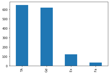
df1.BsmtQual.value_counts()
#df.groupby(['BsmtQual'])['BsmtQual'].count()

TA    649
Gd    618
Ex    121
Fa     35
Name: BsmtQual, dtype: int64

df1.BsmtQual.value_counts().plot.bar()

<matplotlib.axes._subplots.AxesSubplot at 0x7fe8df97a750>

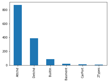
df1.GarageType.value_counts().plot.bar()

<matplotlib.axes._subplots.AxesSubplot at 0x7fe8dfaa4310>

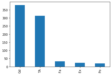
df1.FireplaceQu.value_counts().plot.bar()

<matplotlib.axes._subplots.AxesSubplot at 0x7fe8de336810>

df1.GarageType.mode()[0]

'Attchd'

df1.GarageType.value_counts().index[0]

'Attchd'

def impute_nan(df,variable):
    most_freq_cat=df[variable].value_counts().index[0] #most_freq_cat=df[variable].mode()[0]
    df[variable].fillna(most_freq_cat,inplace=True)

for features in ['BsmtQual','GarageType','FireplaceQu']:
    impute_nan(df1,features)

df1

	BsmtQual	FireplaceQu	GarageType	SalePrice
0	Gd	Gd	Attchd	208500
1	Gd	TA	Attchd	181500
2	Gd	TA	Attchd	223500
3	TA	Gd	Detchd	140000
4	Gd	TA	Attchd	250000
...	...	...	...	...
1455	Gd	TA	Attchd	175000
1456	Gd	TA	Attchd	210000
1457	TA	Gd	Attchd	266500
1458	TA	Gd	Attchd	142125
1459	TA	Gd	Attchd	147500

1460 rows × 4 columns

df1.isna().sum()

BsmtQual       0
FireplaceQu    0
GarageType     0
SalePrice      0
dtype: int64

df1.FireplaceQu.value_counts().plot.bar()

<matplotlib.axes._subplots.AxesSubplot at 0x7fe8de7459d0>

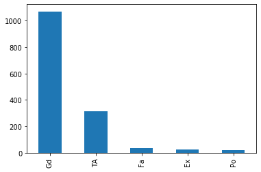
• As FireplaceQu has large missing values (~47%), imputing the same with mode might distort the relationship of FireplaceQu with other variable. So it is not a good practice to impute with mode in case where there is higher percentage of missing values

Advantages

1. Easy and faster way to implement

Disadvantages

1. Since we are using more frequent label, it may use them in an over-represented way if there are many NANs.
2. It distorts the relation of the most frequent label.

2. Adding a variable to capture NAN

df2=pd.read_csv('Datasets/House_prices/train.csv',usecols=['BsmtQual','FireplaceQu','GarageType','SalePrice'])

df2['BsmtQual_NAN']=np.where(df2.BsmtQual.isna(),1,0)

impute_nan(df2,'BsmtQual')

df2.head()

	BsmtQual	FireplaceQu	GarageType	SalePrice	BsmtQual_NAN
0	Gd	NaN	Attchd	208500	0
1	Gd	TA	Attchd	181500	0
2	Gd	TA	Attchd	223500	0
3	TA	Gd	Detchd	140000	0
4	Gd	TA	Attchd	250000	0

• we are capturing the importance of missing value (here by using a variable+_NAN column) and also imputing the column with mode (most frequnent category)
• Since we are capturing the importance of missing values, we can also apply this to the column having higher percentage of missing value (i.e. FireplaceQu)

df2['FireplaceQu_NAN']=np.where(df2.FireplaceQu.isna(),1,0)

impute_nan(df2,'FireplaceQu')

df2

	BsmtQual	FireplaceQu	GarageType	SalePrice	BsmtQual_NAN	FireplaceQu_NAN
0	Gd	Gd	Attchd	208500	0	1
1	Gd	TA	Attchd	181500	0	0
2	Gd	TA	Attchd	223500	0	0
3	TA	Gd	Detchd	140000	0	0
4	Gd	TA	Attchd	250000	0	0
...	...	...	...	...	...	...
1455	Gd	TA	Attchd	175000	0	0
1456	Gd	TA	Attchd	210000	0	0
1457	TA	Gd	Attchd	266500	0	0
1458	TA	Gd	Attchd	142125	0	1
1459	TA	Gd	Attchd	147500	0	1

1460 rows × 6 columns

3. Replace NAN with a new category

we use it if we have more frequent categories

df3=pd.read_csv('Datasets/House_prices/train.csv',usecols=['BsmtQual','FireplaceQu','GarageType','SalePrice'])

def impute_nan_new_cat(df,variable):
    df[variable+"_newvar"]=df[variable].fillna('Missing_'+variable)

for features in ['BsmtQual','GarageType','FireplaceQu']:
    impute_nan_new_cat(df3,features)

df3

	BsmtQual	FireplaceQu	GarageType	SalePrice	BsmtQual_newvar	GarageType_newvar	FireplaceQu_newvar
0	Gd	NaN	Attchd	208500	Gd	Attchd	Missing_FireplaceQu
1	Gd	TA	Attchd	181500	Gd	Attchd	TA
2	Gd	TA	Attchd	223500	Gd	Attchd	TA
3	TA	Gd	Detchd	140000	TA	Detchd	Gd
4	Gd	TA	Attchd	250000	Gd	Attchd	TA
...	...	...	...	...	...	...	...
1455	Gd	TA	Attchd	175000	Gd	Attchd	TA
1456	Gd	TA	Attchd	210000	Gd	Attchd	TA
1457	TA	Gd	Attchd	266500	TA	Attchd	Gd
1458	TA	NaN	Attchd	142125	TA	Attchd	Missing_FireplaceQu
1459	TA	NaN	Attchd	147500	TA	Attchd	Missing_FireplaceQu

1460 rows × 7 columns