Feature Engineering 1 - Missing values - Numerical

Missing Values - Feature Engineering

Lifecycle of Data Science projects

1. Data Collection Strategy
   • from company side
   • 3rd party API’s
   • Surveys
2. Featue Engineering
   • handling missing values

why are there missing values? - In case of surveys, people might have not filled the values - some input error while uploading numbers into system

• In Data Science projects -> Data should be collected from multiple sources

• Types of data that might be missings:-

  • Continuous data
    • Discrete continuous data (e.g age which will have integral value)
    • Continuous data (e.g. height)
  • categorial data

What are different types of Missing data?

1. Missing completely at random (MCAR)

   • a variable is missing completely at random (MCAR) if the probability of being missing is same for all the observations. When data is MCAR, there is absolutely no relationship between the data missing and any other values,observed or missing, within dataset. In other words, those missing data points are a random subset of the data. There is nothing systematic going on that makes some data more likely to be missing than other. if values for observation are missing completely at random, then disregarding those cases would not bias the inferences made.

import pandas as pd
import numpy as np
import matplotlib.pyplot as plt
import seaborn as sns
%matplotlib inline

df=pd.read_csv('Datasets/Titanic/train.csv')

df.head()

	PassengerId	Survived	Pclass	Name	Sex	Age	SibSp	Parch	Ticket	Fare	Cabin	Embarked
0	1	0	3	Braund, Mr. Owen Harris	male	22.0	1	0	A/5 21171	7.2500	NaN	S
1	2	1	1	Cumings, Mrs. John Bradley (Florence Briggs Th...	female	38.0	1	0	PC 17599	71.2833	C85	C
2	3	1	3	Heikkinen, Miss. Laina	female	26.0	0	0	STON/O2. 3101282	7.9250	NaN	S
3	4	1	1	Futrelle, Mrs. Jacques Heath (Lily May Peel)	female	35.0	1	0	113803	53.1000	C123	S
4	5	0	3	Allen, Mr. William Henry	male	35.0	0	0	373450	8.0500	NaN	S

df.isna().sum() #Number of missing values in each columns

PassengerId      0
Survived         0
Pclass           0
Name             0
Sex              0
Age            177
SibSp            0
Parch            0
Ticket           0
Fare             0
Cabin          687
Embarked         2
dtype: int64

• We can sense that there might be relationship between age and Cabin missing values as the person whose age is unknown cabin seems unknown for them, or person having null values in Age and Cabin may not have survived.

• Missing values of Embarked seems MCAR.

df[df.Embarked.isna()]

	PassengerId	Survived	Pclass	Name	Sex	Age	SibSp	Parch	Ticket	Fare	Cabin	Embarked
61	62	1	1	Icard, Miss. Amelie	female	38.0	0	0	113572	80.0	B28	NaN
829	830	1	1	Stone, Mrs. George Nelson (Martha Evelyn)	female	62.0	0	0	113572	80.0	B28	NaN

1. Missing data not at random (MNAR) : Systematic missing value

   • There is absolutely some relationship between the data missing and any other values, observed or missing, within the dataset.

df[df.Cabin.isna()]

	PassengerId	Survived	Pclass	Name	Sex	Age	SibSp	Parch	Ticket	Fare	Cabin	Embarked
0	1	0	3	Braund, Mr. Owen Harris	male	22.0	1	0	A/5 21171	7.2500	NaN	S
2	3	1	3	Heikkinen, Miss. Laina	female	26.0	0	0	STON/O2. 3101282	7.9250	NaN	S
4	5	0	3	Allen, Mr. William Henry	male	35.0	0	0	373450	8.0500	NaN	S
5	6	0	3	Moran, Mr. James	male	NaN	0	0	330877	8.4583	NaN	Q
7	8	0	3	Palsson, Master. Gosta Leonard	male	2.0	3	1	349909	21.0750	NaN	S
...	...	...	...	...	...	...	...	...	...	...	...	...
884	885	0	3	Sutehall, Mr. Henry Jr	male	25.0	0	0	SOTON/OQ 392076	7.0500	NaN	S
885	886	0	3	Rice, Mrs. William (Margaret Norton)	female	39.0	0	5	382652	29.1250	NaN	Q
886	887	0	2	Montvila, Rev. Juozas	male	27.0	0	0	211536	13.0000	NaN	S
888	889	0	3	Johnston, Miss. Catherine Helen "Carrie"	female	NaN	1	2	W./C. 6607	23.4500	NaN	S
890	891	0	3	Dooley, Mr. Patrick	male	32.0	0	0	370376	7.7500	NaN	Q

687 rows × 12 columns

#df['cabin_null']=df['Cabin'].apply(lambda x: 0 if x.isna() else 1)
df['cabin_null']=np.where(df.Cabin.isna(),1,0)

df[['Cabin','cabin_null']].head()

	Cabin	cabin_null
0	NaN	1
1	C85	0
2	NaN	1
3	C123	0
4	NaN	1

#find percentage of null values
df['cabin_null'].mean() #Alternate -> df.Cabin.isna().mean()

0.7710437710437711

df.columns

Index(['PassengerId', 'Survived', 'Pclass', 'Name', 'Sex', 'Age', 'SibSp',
       'Parch', 'Ticket', 'Fare', 'Cabin', 'Embarked', 'cabin_null'],
      dtype='object')

Trying to figure out relationship of Cabin missing value with Survived column as we expect there should be less missing values for survived person

df.groupby('Survived').mean().cabin_null

Survived
0    0.876138
1    0.602339
Name: cabin_null, dtype: float64

1. Missing at Random (MAR)

   • The probability of the missing values with respect to various features -> this will be almost same in the whole dataset.
   • When the msising values have no relation with any other column but have relation with the column in which the value is missing
   • e.g. Men hiding their salary, women hiding their age. (Kind of trend being analysed but not dependent to other variable)

All the techniques of handling missing values :-

1. Mean/Median/Mode replacement
2. Random Sample Imputation
3. Capturing NAN values with a new feature
4. End of Distribution imputation
5. Arbitrary imputation
6. Frequent categories imputation

1. Mean/Median/Mode imputation

When should we apply this?

• Mean/median imputation has the assumption that the data are missing completely at random (MCAR).
• Solve this by replacing the NAN with most frequent occurence of the variable.
• To overcome outlier we can use media/mode instead of mean.

df1=pd.read_csv('Datasets/Titanic/train.csv',usecols=['Age','Fare','Survived'])

df1.head()

	Survived	Age	Fare
0	0	22.0	7.2500
1	1	38.0	71.2833
2	1	26.0	7.9250
3	1	35.0	53.1000
4	0	35.0	8.0500

#Lets go and see the percentage of missing values
df1.isna().mean()

Survived    0.000000
Age         0.198653
Fare        0.000000
dtype: float64

def impute_nan(df,variable,method):
    if method=='median':
        value=df[variable].median()
    elif method=='mean':
        value=df[variable].mean()
    elif method=='mode':
        value=df[variable].mode()
    df[variable+"_"+method]=df[variable].fillna(value)

impute_nan(df1,'Age','median')

impute_nan(df1,'Age','mode')

impute_nan(df1,'Age','mean')

df1[df1.Age.isna()]

	Survived	Age	Fare	Age_median	Age_mode	Age_mean
5	0	NaN	8.4583	28.0	NaN	29.699118
17	1	NaN	13.0000	28.0	NaN	29.699118
19	1	NaN	7.2250	28.0	NaN	29.699118
26	0	NaN	7.2250	28.0	NaN	29.699118
28	1	NaN	7.8792	28.0	NaN	29.699118
...	...	...	...	...	...	...
859	0	NaN	7.2292	28.0	NaN	29.699118
863	0	NaN	69.5500	28.0	NaN	29.699118
868	0	NaN	9.5000	28.0	NaN	29.699118
878	0	NaN	7.8958	28.0	NaN	29.699118
888	0	NaN	23.4500	28.0	NaN	29.699118

177 rows × 6 columns

• Now we can check whether the standard deviation of age column changed if we compare the same with age_median

print('Age StdDev :-',df1.Age.std())
print('Age_median StdDev :-',df1.Age_median.std())

Age StdDev :- 14.526497332334044
Age_median StdDev :- 13.019696550973194

• Now we can check distributiojn of Age_median w.r.t. Age column using matplotlib

fig=plt.figure(figsize=(10,7))
ax=fig.add_subplot(111)
df1['Age'].plot(kind='kde',ax=ax)
df1.Age_median.plot(kind='kde',ax=ax,color='red')
lines,labels=ax.get_legend_handles_labels()
ax.legend(lines,labels,loc='best')

<matplotlib.legend.Legend at 0x7f98f26f7f10>

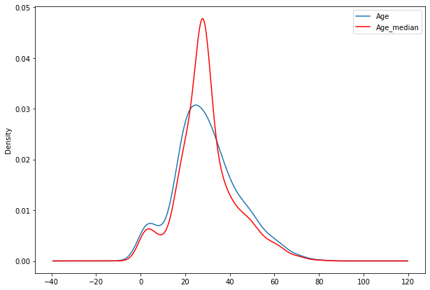
Advantages and disadvantages of Mean/Median imputations

Advantages :-

1. Easy to implement.
2. Robust to outliers (Median only).
3. Faster way to obtain complete datasets. #### Disadvantages :-
1. Change or distortion in the original variance/standard deviation.
2. It impacts correlation

2. Random Sample Imputation

Aim: Random sample imputation consists of taking random observation from the dataset and we use this observation to replace NAN value.

When shout it be used?

It assumes that data are missing completely at random (MCAR).

df2=pd.read_csv('Datasets/Titanic/train.csv',usecols=['Survived','Age','Fare'])

df2.head()

	Survived	Age	Fare
0	0	22.0	7.2500
1	1	38.0	71.2833
2	1	26.0	7.9250
3	1	35.0	53.1000
4	0	35.0	8.0500

df2.isnull().sum()

Survived      0
Age         177
Fare          0
dtype: int64

df2.isnull().mean()

Survived    0.000000
Age         0.198653
Fare        0.000000
dtype: float64

df['Age'].dropna().sample(df.Age.isna().sum(),random_state=0)

423    28.00
177    50.00
305     0.92
292    36.00
889    26.00
       ...  
539    22.00
267    25.00
352    15.00
99     34.00
689    15.00
Name: Age, Length: 177, dtype: float64

def impute_nan_rand(df,variable,method):
    if method!='random':
        if method=='median':
            value=df[variable].median()
        elif method=='mean':
            value=df[variable].mean()
        elif method=='mode':
            value=df[variable].mode()
        df[variable+"_"+method]=df[variable].fillna(value)
    else:
        ## Just to itroduce variable_random column which will be updated later
        df[variable+"_random"]=df[variable]
        ## it will have the random sample to fill NAN value
        random_sample=df['Age'].dropna().sample(df.Age.isna().sum(),random_state=0)
        ## pandas need to have same index in order to merge the datasets
        random_sample.index=df[df[variable].isna()].index
        #updating variable_random column with random sample for NAN values
        df.loc[df[variable].isna(),variable+'_random']=random_sample

impute_nan_rand(df2,'Age','random')

df2

	Survived	Age	Fare	Age_random
0	0	22.0	7.2500	22.0
1	1	38.0	71.2833	38.0
2	1	26.0	7.9250	26.0
3	1	35.0	53.1000	35.0
4	0	35.0	8.0500	35.0
...	...	...	...	...
886	0	27.0	13.0000	27.0
887	1	19.0	30.0000	19.0
888	0	NaN	23.4500	15.0
889	1	26.0	30.0000	26.0
890	0	32.0	7.7500	32.0

891 rows × 4 columns

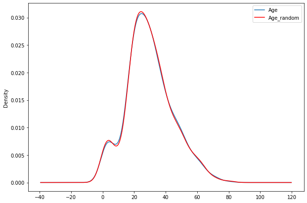
print('Age StdDev :-',df2.Age.std())
print('Age_random StdDev :-',df2.Age_random.std())

Age StdDev :- 14.526497332334044
Age_random StdDev :- 14.5636540895687

fig=plt.figure(figsize=(10,7))
ax=fig.add_subplot(111)
df2['Age'].plot(kind='kde',ax=ax)
df2.Age_random.plot(kind='kde',ax=ax,color='red')
lines,labels=ax.get_legend_handles_labels()
ax.legend(lines,labels,loc='best')

<matplotlib.legend.Legend at 0x7f98f3f8da10>

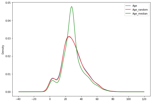
impute_nan_rand(df2,'Age','median')

fig=plt.figure(figsize=(10,7))
ax=fig.add_subplot(111)
df2['Age'].plot(kind='kde',ax=ax)
df2.Age_random.plot(kind='kde',ax=ax,color='red')
df2.Age_median.plot(kind='kde',ax=ax,color='green')
lines,labels=ax.get_legend_handles_labels()
ax.legend(lines,labels,loc='best')

<matplotlib.legend.Legend at 0x7f98f410bd50>

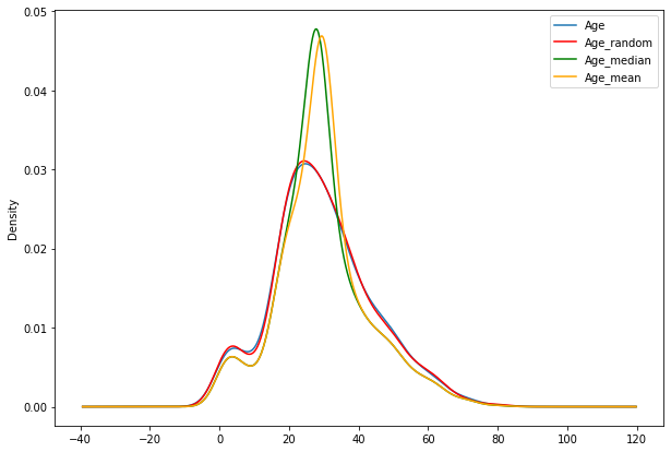
impute_nan_rand(df2,'Age','mean')

fig=plt.figure(figsize=(10,7))
ax=fig.add_subplot(111)
df2['Age'].plot(kind='kde',ax=ax)
df2.Age_random.plot(kind='kde',ax=ax,color='red')
df2.Age_median.plot(kind='kde',ax=ax,color='green')
df2.Age_mean.plot(kind='kde',ax=ax,color='orange')
lines,labels=ax.get_legend_handles_labels()
ax.legend(lines,labels,loc='best')

<matplotlib.legend.Legend at 0x7f98f40e2310>

Advantages

1. Easy to implement
2. Less distortion in variance or standard deviation

Disadvantages

1. In every situation randomness won’t work

3. Capturing NAN values with a new feature

It works well if the data are missing completely not at random (MNAR).

df3=pd.read_csv('Datasets/Titanic/train.csv',usecols=['Survived','Age','Fare'])

df3.head()

	Survived	Age	Fare
0	0	22.0	7.2500
1	1	38.0	71.2833
2	1	26.0	7.9250
3	1	35.0	53.1000
4	0	35.0	8.0500

#Just to flag the missing value, from this we can identify which row has been imputed from missing value
df3['Age_NAN']=np.where(df3.Age.isna(),1,0)

df3.Age_NAN

0      0
1      0
2      0
3      0
4      0
      ..
886    0
887    0
888    1
889    0
890    0
Name: Age_NAN, Length: 891, dtype: int64

df3

	Survived	Age	Fare	Age_NAN
0	0	22.0	7.2500	0
1	1	38.0	71.2833	0
2	1	26.0	7.9250	0
3	1	35.0	53.1000	0
4	0	35.0	8.0500	0
...	...	...	...	...
886	0	27.0	13.0000	0
887	1	19.0	30.0000	0
888	0	NaN	23.4500	1
889	1	26.0	30.0000	0
890	0	32.0	7.7500	0

891 rows × 4 columns

df3['Age'].fillna(df3.Age.median(),inplace=True)

df3

	Survived	Age	Fare	Age_NAN
0	0	22.0	7.2500	0
1	1	38.0	71.2833	0
2	1	26.0	7.9250	0
3	1	35.0	53.1000	0
4	0	35.0	8.0500	0
...	...	...	...	...
886	0	27.0	13.0000	0
887	1	19.0	30.0000	0
888	0	28.0	23.4500	1
889	1	26.0	30.0000	0
890	0	32.0	7.7500	0

891 rows × 4 columns

Advantages

1. Easy to implement
2. Captures the importance of missing values. (Age_NAN column giving importance to missing value as it is 1 for NAN cases)

Disadvantages

1. Creating additional features, as number of features which have missing values increases we need to create same number of additional features. (Curse of Dimensionality)

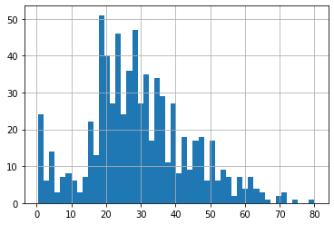
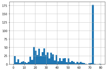
4. End of Distribution imputation

If there is suspicion that the missing value is not at random then capturing that information is important. In this scenario, one would want to replace missing data with values that are at the tails of the distribution of the variable.

df4=pd.read_csv('Datasets/Titanic/train.csv',usecols=['Survived','Age','Fare'])
df4.head()

	Survived	Age	Fare
0	0	22.0	7.2500
1	1	38.0	71.2833
2	1	26.0	7.9250
3	1	35.0	53.1000
4	0	35.0	8.0500

df4.Age.hist(bins=50)

<matplotlib.axes._subplots.AxesSubplot at 0x7f98f3887750>

#Mean
df4.Age.mean()

29.69911764705882

#Standard deviation
df4.Age.std()

14.526497332334044

sns.boxplot('Age',data=df4)

<matplotlib.axes._subplots.AxesSubplot at 0x7f98f4e01ed0>

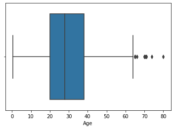
• In this dataset we have only right side outliers, therefore we will impute the missing values from roght extremem values

#Picking values from right end of distribution -> mean+3*standard_deviation
df4.Age.mean()+3*df4.Age.std()

73.27860964406095

def impute_nan_extreme(df,variable,method):
    if method=='random':
        ## Just to itroduce variable_random column which will be updated later
        df[variable+"_random"]=df[variable]
        ## it will have the random sample to fill NAN value
        random_sample=df['Age'].dropna().sample(df.Age.isna().sum(),random_state=0)
        ## pandas need to have same index in order to merge the datasets
        random_sample.index=df[df[variable].isna()].index
        #updating variable_random column with random sample for NAN values
        df.loc[df[variable].isna(),variable+'_random']=random_sample
    elif method=='extreme':
        #getting the right extreme value (mean+3*std_dev)
        value=df[variable].mean()+3*df[variable].std()
        df[variable+"_end_distribution"]=df[variable].fillna(value)
    else:
        if method=='median':
            value=df[variable].median()
        elif method=='mean':
            value=df[variable].mean()
        elif method=='mode':
            value=df[variable].mode()
        df[variable+"_"+method]=df[variable].fillna(value)

impute_nan_extreme(df4,'Age','extreme')

df4

	Survived	Age	Fare	Age_end_distribution
0	0	22.0	7.2500	22.00000
1	1	38.0	71.2833	38.00000
2	1	26.0	7.9250	26.00000
3	1	35.0	53.1000	35.00000
4	0	35.0	8.0500	35.00000
...	...	...	...	...
886	0	27.0	13.0000	27.00000
887	1	19.0	30.0000	19.00000
888	0	NaN	23.4500	73.27861
889	1	26.0	30.0000	26.00000
890	0	32.0	7.7500	32.00000

891 rows × 4 columns

impute_nan_extreme(df4,'Age','median')

df4

	Survived	Age	Fare	Age_end_distribution	Age_median
0	0	22.0	7.2500	22.00000	22.0
1	1	38.0	71.2833	38.00000	38.0
2	1	26.0	7.9250	26.00000	26.0
3	1	35.0	53.1000	35.00000	35.0
4	0	35.0	8.0500	35.00000	35.0
...	...	...	...	...	...
886	0	27.0	13.0000	27.00000	27.0
887	1	19.0	30.0000	19.00000	19.0
888	0	NaN	23.4500	73.27861	28.0
889	1	26.0	30.0000	26.00000	26.0
890	0	32.0	7.7500	32.00000	32.0

891 rows × 5 columns

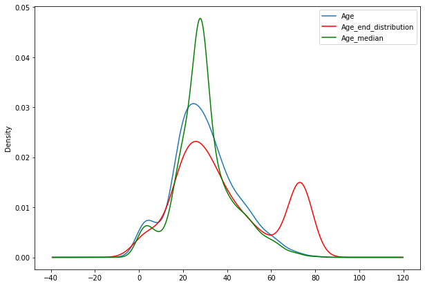
fig=plt.figure(figsize=(10,7))
ax=fig.add_subplot(111)
df4['Age'].plot(kind='kde',ax=ax)
df4.Age_end_distribution.plot(kind='kde',ax=ax,color='red')
df4.Age_median.plot(kind='kde',ax=ax,color='green')
lines,labels=ax.get_legend_handles_labels()
ax.legend(lines,labels,loc='best')

<matplotlib.legend.Legend at 0x7f98f4ee6350>

df4.Age.hist(bins=50)

<matplotlib.axes._subplots.AxesSubplot at 0x7f98f5ebfc10>

df4.Age_median.hist(bins=50)

<matplotlib.axes._subplots.AxesSubplot at 0x7f98f58e5f50>

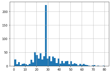
df4.Age_end_distribution.hist(bins=50)

<matplotlib.axes._subplots.AxesSubplot at 0x7f98f5a84f10>

sns.boxplot('Age_end_distribution',data=df4)

<matplotlib.axes._subplots.AxesSubplot at 0x7f98f6042190>

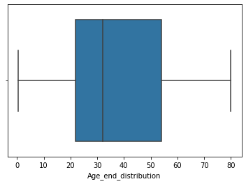
• we can see that there is no more outliers after end of distribution imputation.
• We can observe skewness in the distribution after imputation.

Advantages

1. Easy to implement
2. Captures the importance of missing values if there is one

Disadvantages

1. Distorts the original distribution of the variable
2. If missingness is not important, it may mask the predictive power of the original variable by distorting its distribution.
3. If number of NAN is big, it will mask true outliers in the distribution
4. If the number of NAN is small, the replaced NAN may be considered as outlier and pre-processed in subsequent steps of feature engineering

Note

• if we are working in real world environment only one type of feature engineering will not be sufficient, we need to show all the observation/scenarios to the stakeholders.

5. Arbitrary imputation

• It consists of replacing NAN by an arbitrary value
• This technique was derived from kaggle competetions

df5=pd.read_csv('Datasets/Titanic/train.csv',usecols=['Survived','Age','Fare'])
df5.head()

	Survived	Age	Fare
0	0	22.0	7.2500
1	1	38.0	71.2833
2	1	26.0	7.9250
3	1	35.0	53.1000
4	0	35.0	8.0500

df5.Age.hist(bins=50)

<matplotlib.axes._subplots.AxesSubplot at 0x7f98f63dc250>

Arbitrary values :-

• It should not be the more frequently present in data
• we can either use right end (or > right end) or left end (or < left end)

def impute_arbitrary(df,variable):
    df[variable+"_rightend"]=df[variable].fillna(df[variable].max()+20)
    df[variable+"_leftend"]=df[variable].fillna(df[variable].min())

impute_arbitrary(df5,'Age')

df5

	Survived	Age	Fare	Age_rightend	Age_leftend
0	0	22.0	7.2500	22.0	22.00
1	1	38.0	71.2833	38.0	38.00
2	1	26.0	7.9250	26.0	26.00
3	1	35.0	53.1000	35.0	35.00
4	0	35.0	8.0500	35.0	35.00
...	...	...	...	...	...
886	0	27.0	13.0000	27.0	27.00
887	1	19.0	30.0000	19.0	19.00
888	0	NaN	23.4500	100.0	0.42
889	1	26.0	30.0000	26.0	26.00
890	0	32.0	7.7500	32.0	32.00

891 rows × 5 columns

Advantages

1. Easy to implement
2. Captures the importance of missing values if there is one

Disadvantages

1. Distorts the original distribution of the variable
2. If missingness is not important, it may mask the predictive power of the original variable by distorting its distribution.
3. Hard to decide which value to use